Practical Process Control Part 9: Resolving Potential Level Control Problems

Myke King continues his detailed series on process control, seeking to inspire chemical engineers to exploit untapped opportunities for improvement

IN THE last article we developed tuning formulae for both tight and averaging level control, using a selection of the commonly available control algorithms. But the assumption behind all the calculations is that we can predict the change in level from the change in flow. Strictly, we predict the change in volume but assume that this is linearly related to level. This is, of course, perfectly valid if the vessel is a vertical cylinder. But for horizontal vessels, with dished ends, this is not exactly the case.

Ranging the level transmitter

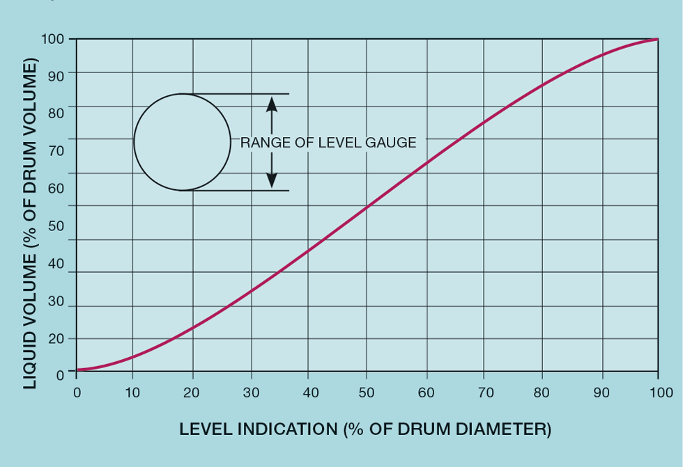
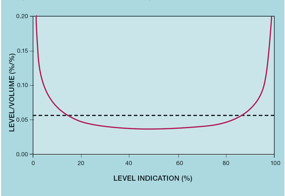
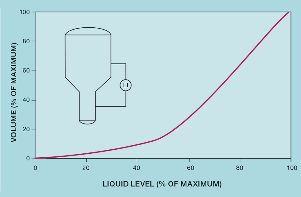
Figure 1 shows, for such a vessel, the relationship between volume and level. It is drawn on the basis that the level gauge is ranged over the full height of the drum. At the extremes, the process gain between level and flow will be much larger than that near the centreline of the vessel. Relatively little liquid volume is required to make large changes in level. This is illustrated in Figure 2, which plots the ratio of level to volume. It is this ratio that determines the process gain. Irrespective of the vessel dimensions, its minimum value is 0.038.

Empirically, a variation of up to ±20% in process gain would be unnoticeable in terms of controller performance. So, provided the ratio remains less than 0.057 (1.5 x 0.038), then it will stay within 20% of the average of 0.048. By measuring over a narrower range, avoiding the very top and bottom of the vessel, the relationship will become more linear. As the figure shows, the maximum range is around 15 to 85% of the drum height. While we want to use all the available surge capacity, sacrificing 30% of the drum’s height loses only about 16% of the total vessel volume.

Linearisation

While it should be obvious that experienced control engineers are routinely involved in process design, this is often not the case. It is quite likely that the engineer is faced with the problem of dealing with, what was, avoidable non-linearity. The solution is to, in the control system, convert the level indication from % of gauge height to % of working volume. Done rigorously, the equations involved are complex. If h₀ is the distance from the bottom of the vessel to 0% on the level gauge, then the volume of (V₀) this section of the drum is given by

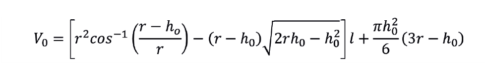
The second term allows for the dished ends; r is the drum radius and l its length, measured as the distance between the tan lines.

We can write a similar equation for V₁₀₀, based on h₁₀₀ – the distance from the bottom of the drum to the 100% on the level gauge. V₀ and _V100 are constants (the difference between them is V), and they can be calculated off-line. However, the current volume (V_now) has to be calculated on-line from the height (h_now) of the liquid, again measured from the bottom of the drum – where h_now is determined from the level indication (L).

We then calculate the process variable (PV) that will be used by the level controller.

This is an example of signal conditioning. In this case, it appears to the process operator as a conventional level measurement. However, the calculation, as written, may not be practical. For example, the control system may not support the cos^-1 function.

Curve fitting

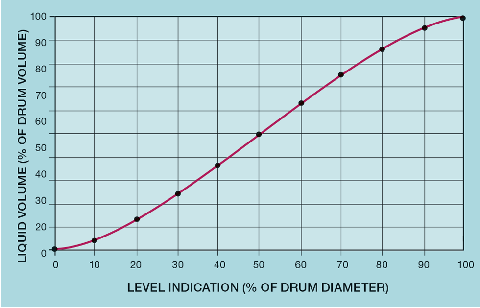
Instead, we can develop a curve-fitting approach. This involves using the formulae above to calculate the % volume (V) at different % level indications (L), say at 10% intervals. This is known as a strapping table. We then fit (for example) a cubic function to these points.

We must apply some conditions to this equation. Firstly, we want PV to be 0 when L is 0, and so a₀ must be 0. Similarly, we want PV to be 100 when L is 100. So,

The predicted level (V^*) is given by

We can use Excel Solver to derive a₂ and a₃ by minimising ∑(V – V*)². In the case where the level gauge covers the whole height of the drum, a₂ is 0.0228 and a₃ is -0.000152. Figure 3 shows that this fits the strapping points well.

An extreme example of non-linearity is included as Figure 4. If a suitable polynomial cannot be developed, then the strapping table itself would be used – interpolating between points. Some distributed control systems (DCSs) support this feature. In others, it would require some custom coding.

Integrating process

Not all level controllers lend themselves to the design approach we covered in the last article. Consider that in Figure 5. As we’ll see later in the next article, covering level control of distillation columns, this scheme should preferably be avoided. However, if the bottom product flow is a small fraction of the feed, we can’t adopt the normal approach of using it to control the column level. The problem we now have with tuning, is that there isn’t a predictable relationship between the level and its manipulated flow.

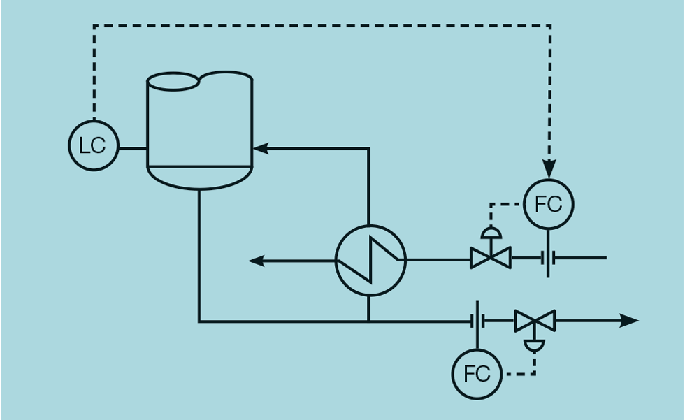
Theoretically we could derive this relationship using the enthalpy of steam and the heat of vaporisation for water, but it is likely to be unreliable. Secondly, our approach so far has ignored process dynamics. We (reasonably) assumed that the level begins to change immediately following a change in flow. In this case the reboiler, because it has thermal capacity, will introduce a significant lag.

Further, liquid level is not the only example of an integrating process. Consider a pressure controller on a steam header. If we increase boiler duty to produce more steam but consumption is fixed, then the pressure will show integrating behaviour. We therefore need a way of characterising the process dynamics and then using these to tune the controller. As we did for the self-regulating process (See TCE 981), we can apply a curve-fitting approach to identify the relationship between the process variable (PV) and its manipulated variable (MV). The steady state behaviour of a self-regulating process is governed by

An integrating process does not reach a new steady state; its behaviour is governed by

Differentiating

So instead of fitting PV to MV, we fit the rate of change of PV to MV. Actually, we fit ΔPV to MV×ts, where ts is the data collection interval.

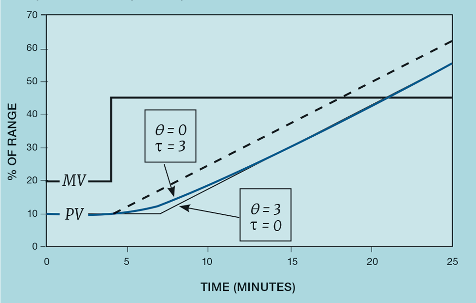
Integrating processes have simpler dynamics. Figure 6 shows, as the dashed line, the behaviour of an integrating process with no deadtime and no lag (like most liquid levels). Also shown is the effect of adding either a three-minute deadtime or a three-minute lag. Both follow almost the same trend and are, within the accuracy required, interchangeable. The convention is to include only deadtime in the model. So, the predicted PV is given by

We follow the same curve-fitting methodology that we documented in TCE 981. Both PV and MV are converted to % of instrument range. However, unlike self-regulating processes in which the process gain (Kp) is dimensionless, for integrating processes it must have units of reciprocal time. Conventionally we choose min^-1. In other words, when fitting the model, the data collection interval (ts) should be in minutes.

As we have seen before, using this curve-fitting approach allows us to obtain process dynamics from closed loop tests. This is particularly advantageous for integrating processes. The controller ensures that we move from one steady state to another. Indeed, we may not have to execute the test at all. If there is a process historian, it is likely to have recorded routine changes in the setpoint that can be analysed retrospectively. But note that some process historians use data compression to reduce storage requirements. This will distort the dynamics obtained. Data compression should ideally be disabled, if only for the measurements involved. Indeed, given the rapidly falling cost of data storage, it should be disabled for all measurements.

The option to tune a controller on an integrating process is included in the software downloadable from the website (see TCE 983). Note that the tuning criteria applied by the software are designed to deliver tight control. For our column level, this is what is required. Indeed, because of the inherent process lag, the controller would benefit from the inclusion of derivative action – unusual for level control. The software will work for any integrating process including, for example, the steam header pressure example. It will not, however, deliver averaging control or work with the error-squared or gap controller. These require the calculations derived in the previous article.

The topics featured in this series are covered in greater detail in Myke King's book, Process Control – A Practical Approach, published by Wiley in 2016.

---

This is the ninth in a series that provides practical process control advice on how to bolster your processes. To read more, visit the series hub at https://www.thechemicalengineer.com/tags/practical-process-control/

---

Disclaimer: This article is provided for guidance alone. Expert engineering advice should be sought before application.