Practical Process Control Part 6: Derivative Action

Myke King continues his detailed series on process control, seeking to inspire chemical engineers to exploit untapped opportunities for improvement

The majority of controllers in use in the process industry use the PI rather than the PID algorithm. There are several reasons for this. The first is probably that the addition of derivative action to a controller is undervalued by the engineer. Certainly, if simply added to a working PI controller, its advantage will not be immediately obvious. This is not helped by some of the published tuning methods. For example, the Internal Model Control (IMC) method we covered in Issue 983, will give the same response to a setpoint (SP) change for both the PI and the PID algorithm. Other methods, like Cohen-Coon, suggest that derivative action is of no benefit if the deadtime (θ) is small.

To see the benefit of adding derivative action to a working PI controller, the existing tuning constants must be redetermined. If trial-and-error is the tuning method of choice, this is impractical. When performed manually, a three-dimensional search is considerably more difficult than a two-dimensional one.

The other main reason is that derivative action is known to amplify any measurement noise, transmitting it to the control valve and potentially causing its failure. This article aims to address both issues.

Use the ideal PID algorithm

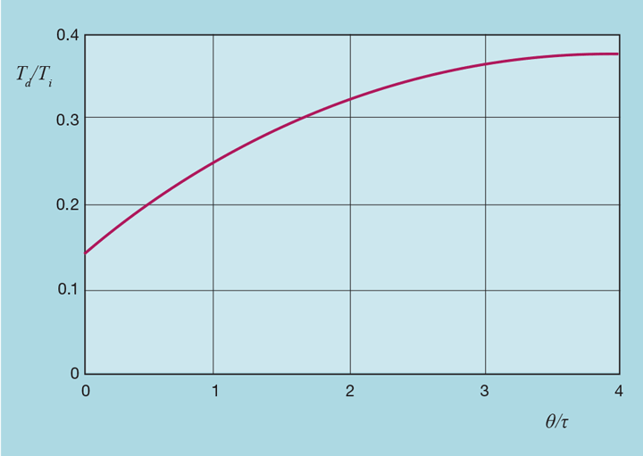
Figure 1 shows the requirement for derivative action, particularly as the deadtime-to-lag ratio (θ/τ) increases. Presented as a fraction of the integral time, it influences our choice of control algorithm. We previously presented (Issue 983) the formulae for converting tuning for the interactive PID algorithm to that for the ideal version. Inverting these formulae gives

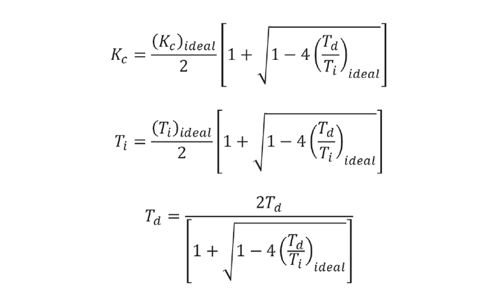
Unlike the conversion in the former direction, there is now the condition that the ratio T_d/T_i in the ideal version cannot exceed 0.25. Figure 1 shows that the required ratio substantially exceeds this value – particularly when θ exceeds τ. Under these circumstances an optimally tuned ideal PID cannot be replaced with an equivalent interactive PID. It gives us a reason to choose the ideal version as our standard.

To see the benefit of adding derivative action to a working PI controller, the existing tuning constants must be redetermined. If trial-and-error is the tuning method of choice, this is impractical

Increase controller gain

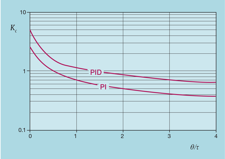
Figure 2 shows the impact that the addition of derivative action has on controller gain. (Note the logarithmic scale.) It typically allows K_c to be increased by about 80%. This is consistent across the range of process dynamics. So why we might think its predictive nature is of little value when the deadtime is small, it still permits us to substantially increase controller gain. In the same way that choosing the I-PD algorithm permits such an increase, it will substantially reduce the impact of process disturbances.

Noise problem

The reluctance to apply derivative action is that it is known to amplify noise. Let’s imagine that the noise in our process value (PV) can be described as a sine wave with frequency f.

Derivative action is based on the derivative of PV

Differentiation increases the amplitude of the noise by a factor of 2πf. The higher the frequency, the greater the amplification. It would not be unusual for noise, say of amplitude 1% of instrument range, to be amplified to the point where the control valve is moved rapidly over its whole range.

Increase the scan interval

Let us consider the effect of the controller scan interval (ts). If we double this, say from 1 to 2 seconds, the amplitude of the noise remains the same but its frequency (as seen by the controller) is halved. This then halves the amplitude produced by derivative action. One of the myths of process control is that the scan interval needs to be very short. Making it so can be counter-productive, requiring filtering (which we’ll show in another article, increases the process lag) and restricting the use of derivative action.

Figure 3 shows the impact of scan interval on controller gain, clearly applying a tuning method that takes account of ts. We’re not suggesting that it ever be increased so much, partly because of the large reduction in K_c. We’re merely demonstrating that it’s possible. The limit is not controllability but how long we are prepared to wait for the controller to scan and so respond to a process disturbance or a SP change.

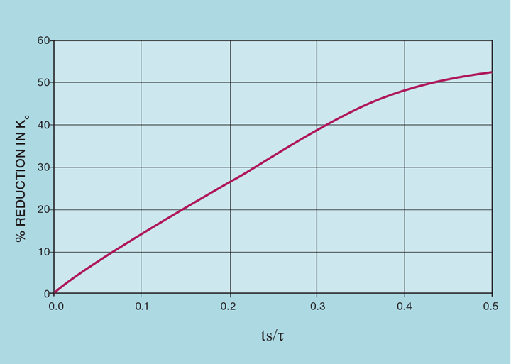
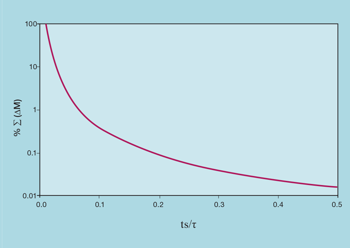
Figure 4 demonstrates the benefit of even small increases. For example, on a process which has a lag of one minute, increasing the scan interval from 1 second to 5 seconds reduces by 97% the effect that noise and derivative action has on total valve travel. This would require a reduction in controller gain of only 2%. Further, if the DCS is operating close to its CPU capacity, increasing scan interval by a few seconds can significantly reduce the system load.