Practical Process Control Part 5: The I-PD Algorithm

Myke King continues his detailed series on process control, seeking to inspire chemical engineers to exploit untapped opportunities for improvement

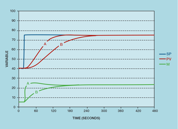
PROBABLY the most misunderstood and underused control algorithm is the I-PD version. Recalling the last issue, it differs from the PI-D in that proportional action is based on the PV (process value) rather than the error. Almost universally, control system vendors, if they do document its purpose, suggest it should be used when only a slow response to set-point (SP) changes is required. However, this can be delivered by any control algorithm, simply by adjusting the tuning. Figure 1 shows, as curve A, a well-tuned controller responding to an SP change. Switching from PI-D to I-PD results in the response shown as curve B. It does, indeed respond more slowly; the algorithm no longer generates the proportional kick, relying solely on the integral action. One can see why the algorithm has the reputation for being slow. But the key issue is that different algorithms require different tuning parameters. It is unreasonable to expect the I-PD to perform well, using tuning designed for the PI-D algorithm.

Benefit of re-tuning

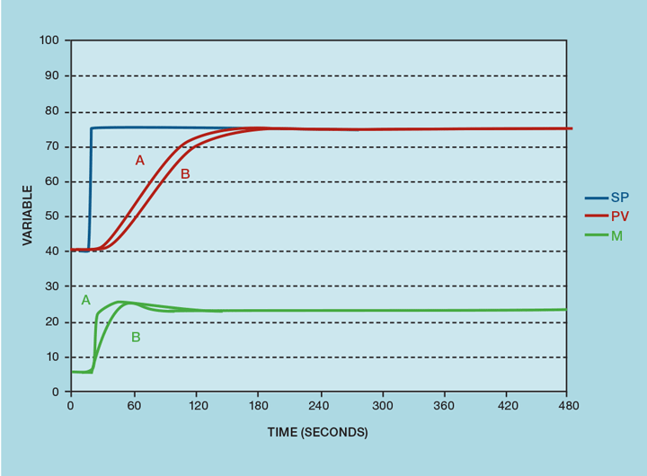
Figure 2 again compares the two algorithms but with the I-PD properly tuned. The lack of proportional kick has been largely compensated for by increasing the controller gain. This hasn’t been achieved by overly aggressive tuning; the manipulated variable (MV) overshoot is the same for both controllers. While the PI-D slightly outperforms the I-PD, it is unlikely this would be noticeable on a real process.

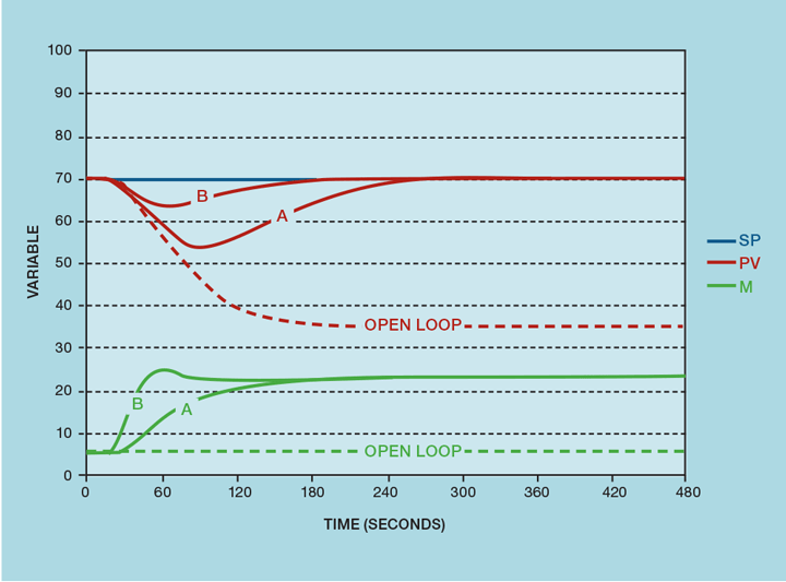
Given the comparable performance still begs the question as to the benefit of the modified algorithm. To understand this, instead of testing the controller with a SP change, we subject it to a load change. This is simply a process disturbance. In the example of our fired heater (Issue 981), this might be an increase in the feed rate. Figure 3 shows the open loop response. With no controller in place, the fuel flow would remain constant and the outlet temperature will reduce to a new steady state. Curve A shows the response of the PI-D controller. Had we not also displayed curve B, the engineer would have been quite content with its behaviour. But we can now see that the I-PD controller returns the process to SP in about half the time. It also reduces the maximum deviation by more than 50%. If the temperature were the main influence on finished product quality, then we will have reduced off-grade production by about 80%. Again, this has not been achieved with aggressive tuning; we stay within the MV overshoot limit.

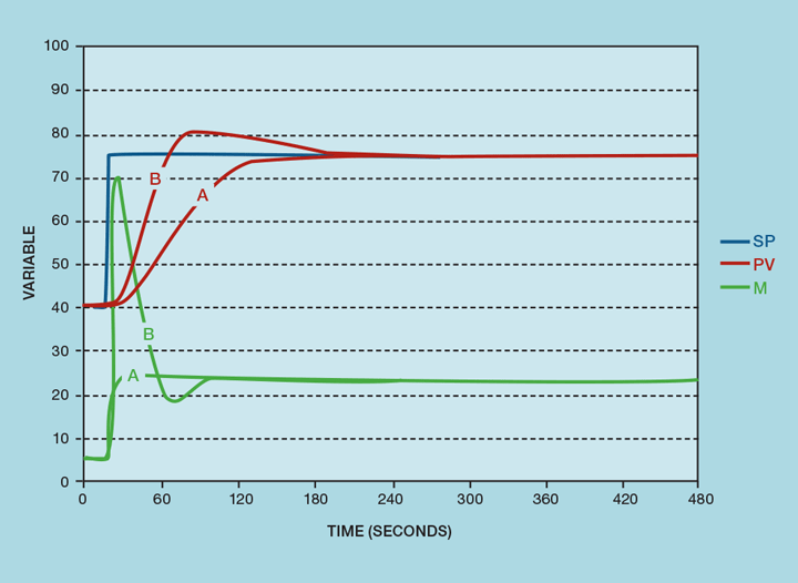
We should emphasise at this point that it is not the change of algorithm that has brought about the improvement. If the SP remains constant, the I-PD and P-ID algorithms perform identically. What has brought about the improvement is the change of tuning. We could have implemented the new tuning in the original controller and seen the same improvement. The change of algorithm is necessary to handle SP changes. This is illustrated in Figure 4. Retaining the P-ID algorithm results in a dangerously aggressive response to the SP change, with MV overshoot approaching 300%.

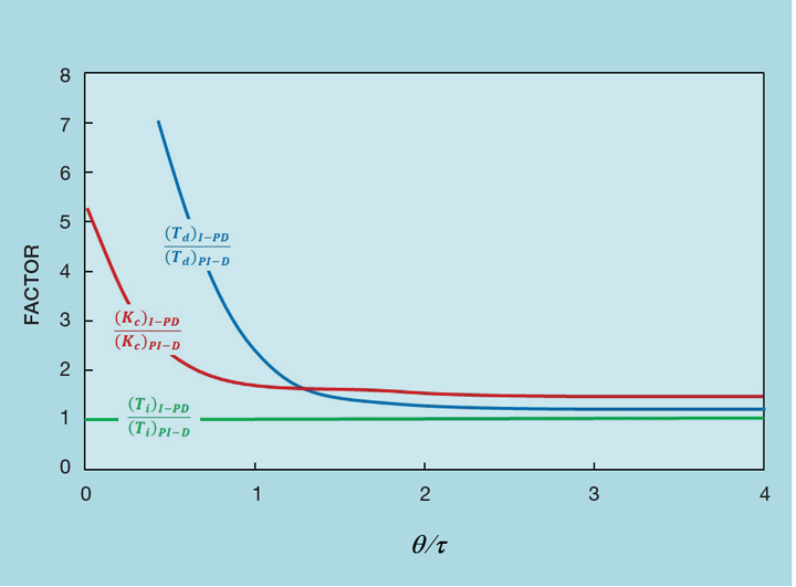
To further emphasise the improvement we can examine precisely just how big the changes to controller tuning can be. Figure 5 shows the factor by which the PID tuning parameters can be increased. At the very least, if the deadtime-to-lag ratio (θ/𝜏) is large, there is potential to increase controller gain (K_c) by 50%. But θ/𝜏 is usually less than 0.5, so it is common that it can be increased threefold. Integral time (T_i) changes little but derivative action (T_d) can also be substantially increased.

It is difficult to overstate the importance of switching to the I-PD algorithm. But firstly we need to consider cascade controllers. In our example, temperature is cascaded to the flow controller; it adjusts the flow SP. (In a future article we will cover the advantages of this approach over the alternative of the temperature controller directly manipulating the fuel valve.) The temperature is the primary (or master) controller, while the flow is the secondary (or slave) controller. The temperature controller will largely need to deal with load changes. We’ve seen that one source of such a disturbance is a change in feed rate. But there are many others – including changes in heater inlet temperature, disturbances to the fuel system (such as header pressure and fuel gas heating value) and variation in heater efficiency (caused by changes to the air-to-fuel ratio). Load disturbances are likely to be far more frequent than SP changes. In many processes the heater temperature SP stays constant for many days.

Automatic algorithm switching