Practical Process Control Part 12: Filters

Myke King explains filters and the benefit of moving away from the standard technique

MANY process measurements are subject to noise. Liquid levels can be turbulent; orifice flow meters will show noise if the flow is mixed phase and pressures may reflect vibration from compressors. Ideally, good process and instrumentation design should have eliminated noise at source. Failing this, filtering can be applied to the measurement prior to its use in a controller. Filtering is an example of signal conditioning.

Implementing a filter, that is a standard feature of the distributed control system (DCS), is a compromise between noise reduction and measurement distortion. Strong filters are effective at noise reduction but can increase both the apparent deadtime and the overall process lag. If these changes are significant, then we must change to slower controller tuning. Typically, this would be required if the deadtime increases by more than 10% or the lag by more than 20%.

On many processes, the degree of filtering typically employed is excessive. Filters are added (wrongly) to make measurement trends look smooth. The criterion that should be used is the amplitude of the signal sent to the actuator – usually a control valve, where excessive valve travel can cause mechanical problems. For example, if the controller gain (K_c) is less than 1 and there is no derivative action (T_d = 0), then the integral action will reduce the noise, potentially to an acceptable amplitude, without the need for filtering.

First order exponential

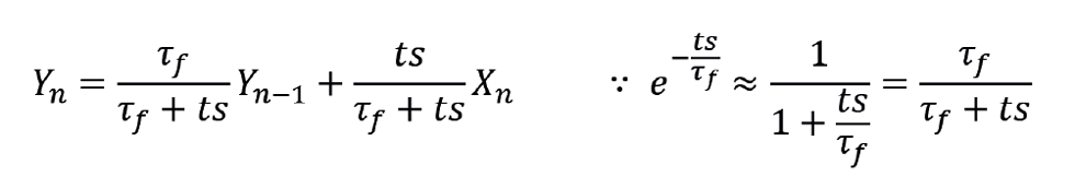
All control systems have the option to filter any measurement – usually by applying the first order exponential filter. First order, because it introduces a single lag ( τ_f) and exponential because of the digital approximation. In general, it takes the form

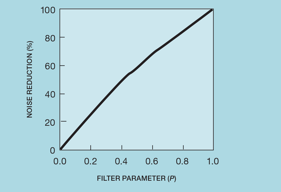
X_n is the current raw measurement, while Y_n is the current filtered value and ts the scan interval. The filter is recursive, in that it uses previous filtered values (in this case just Y_n-1), to determine the current value. Setting P to 0 disables the filter, setting it to 1 blocks any change in the raw measurement. P is selected to give the required level of noise reduction. Figure 1 shows that its effect is approximately linear.

In many systems the engineer will set P directly and is usually free to do so over its whole range. Yokogawa, however, limits the selection to 0, 0.5, 0.75 and 0.85. In other systems the engineer sets τ_f . In Honeywell’s DCS it is the parameter TF which is entered in minutes. In ABB’s it is τ_fil – entered in seconds. The issue with this approach is that P, and hence the level of noise reduction, then depends on the controller scan interval (ts). There are many examples of this being altered, usually associated with a control system upgrade, and the resulting change in noise reduction surprising the engineer. Figure 2 illustrates this. For example, upgrading Honeywell’s TDC2000 to one of its later systems increases the scan interval from 0.33 seconds to 2 seconds. For a 90% noise reduction, TF will have been set to 0.05. 

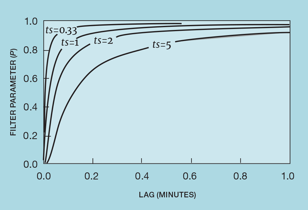
The change in scan interval reduces noise reduction to around 50%. To compensate, TF must be increased to 0.3. In Foxboro’s analog input block (AIN), τ_f  is defined by FTIM, which is entered in minutes. But Foxboro offers three options, selected by defining the parameter FLOP. Setting this to 1 selects the conventional exponential filter, except that its formulation is slightly different

Filtering has been around for much longer than digital control. Most analog instrumentation includes the equivalent of the exponential filter in the field transmitter (for example, this would be a RC network in an electronic analog transmitter). The problem is that this might be adjusted locally, by the instrument technician, unbeknown to the engineer in the control room. This will alter the apparent process dynamics and, if a significant change, will cause control problems. Most sites have procedures that permit such changes only in the control system.

Butterworth

In the Foxboro DCS, setting FLOP = 2 selects the Butterworth filter. In general, Butterworth filters can have an order much greater than 1. That in the Foxboro DCS is second order. The approximation used is

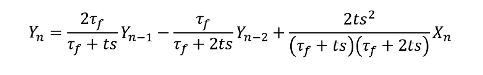
Figure 3 illustrates the advantage over the first order filter. To achieve a noise reduction of 90%, the first order filter requires a value of about 0.9 for P. The Butterworth requires a value of about 0.76. This introduces less additional lag. 

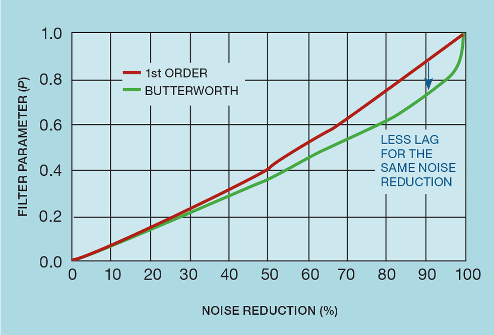
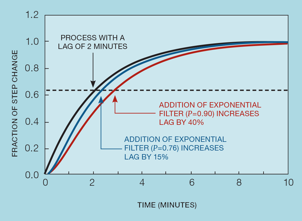
Figure 4 shows the effect of adding these filters to a process that has a lag of two minutes. Using the 63% response time as a measure of lag, the first order filter increases this by about 40% while, for Butterworth, the increase is much less, at 15%. So, if the exponential filter were added, the controller would require retuning while, with the Butterworth, it would not.

On many processes, the degree of filtering typically employed is excessive. Filters are added (wrongly) to make measurement trends look smooth

Moving average

Setting FLOP = 3 in the Foxboro DCS selects the simplest moving average filter, using just the last two raw measurements.

Although not a standard feature in other DCS, it is possible to code a moving average filter relatively easily. Its tuning parameter (N) is simply the number of historical values in calculating the average. So

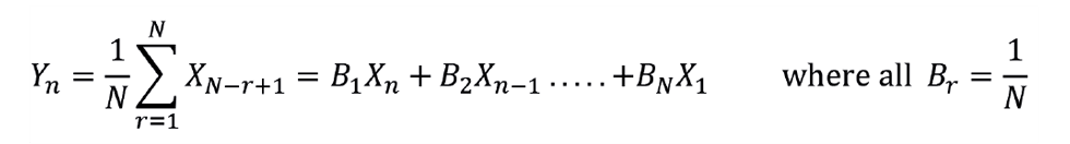
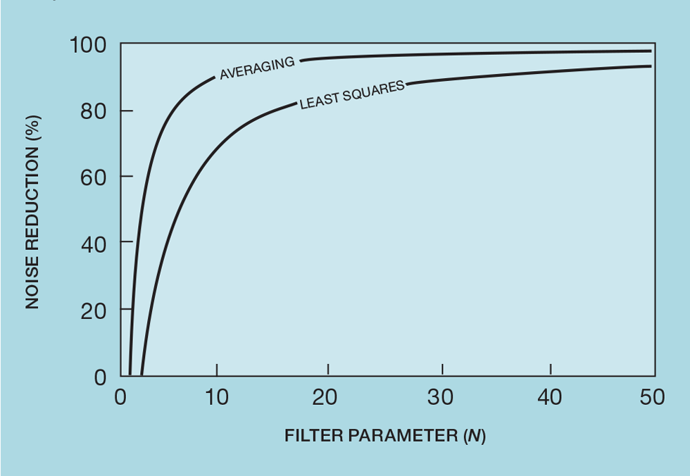
Figure 5 shows its effectiveness. Even with N set to the minimum value of 2, noise is halved. In terms of its effect on process dynamics (following a step change in input), rather than an exponential approach to steady state, the moving average filter produces a ramp of duration N × ts. However, when added to the process lag, the result is indistinguishable from that with the exponential filter. Curve fitting shows we can approximate the filter lag time constant as 0.53N × ts. Given that it is not usually a standard feature of most DCS, the moving average filter offers no advantage over the exponential filter.