Practical Process Control Part 27: Compressor Serge Protection

Myke King explains how prediction, protection and recovery schemes minimise energy costs and safeguard compressors from surge

WHILE some machines can operate in surge for extended periods, others can quickly suffer mechanical problems. And, of course, surge can cause major disruption to the downstream process. While we clearly need a control scheme that will recover quickly from surge, we primarily need it to deliver surge avoidance.

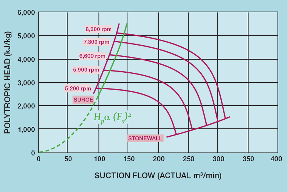
Figure 1 is the example of a compressor map that we saw in the last article, now with the addition of the predicted surge line. To stay above the surge point we need to operate above the minimum flow dictated by this line. While there may be other parameters that can be manipulated, this is most often achieved by recycling some of the gas. This increases the energy consumption. The more accurately we can predict where surge will occur, the closer we can operate to the minimum flow and so reduce operating cost.

Simple anti-surge schemes

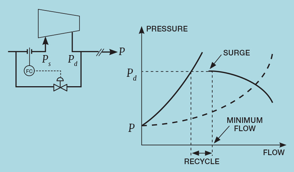
There are many compressors in service that justify only rudimentary surge protection. These will be those operating at a constant speed, compressing a gas of constant composition with little variation in the ratio of discharge pressure to suction pressure. A good example would be the site’s instrument air compressor. Another would be the air blower used to regenerate catalyst in an FCC (fluid catalytic cracker). A candidate scheme would be simple minimum flow protection as shown in Figure 2. It comprises a flow controller with its setpoint set slightly above the surge point – including typically a 15% margin. It is usually based on suction flow, since this is the basis on which the compressor curve would be plotted.

But, since the operating conditions vary little, it would work equally well with a measurement of discharge flow. The recycle remains closed while the flow is above setpoint. This scheme is better applied when the compressor curve is “flat”, since it relies on there being a significant change in flow as the surge point is approached.

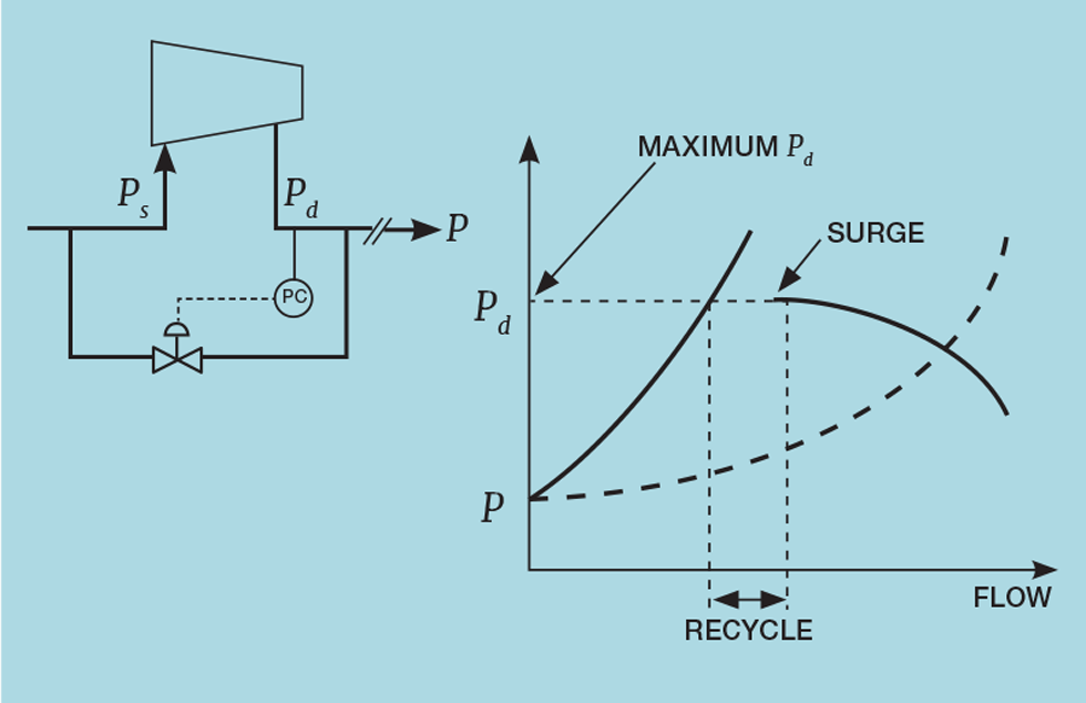
In contrast, Figure 3 presents an alternative scheme for a compressor with a “steep” curve. The discharge pressure now varies significantly as surge is approached so, instead of minimum flow protection, we now set a maximum discharge pressure. 

Surge line

For variable speed machines we can develop a formula that describes the surge line. The simplest form would be the parabola relating the polytropic head (H_p) to the suction flow (F_s), as included in Figure 1:

As noted in TCE 995, the orifice flowmeter formula illustrates how suction flow is derived from the orifice pressure drop (dP) and the gas density at the compressor suction (ρ_s):

So, the polytropic head is related to the pressure drop across the orifice (dP), where f is a linear function:

We developed the definition of polytropic head in the last issue:

Because its calculation includes parameters that can’t readily be measured (such as M, ρ, z, k and η_p), we can’t readily monitor polytropic head. But there are several parameters that are closely related to it. One example is the pressure increase across the machine:

So, the equation of the surge line becomes:

The term (m) is the slope of the surge line. It should pass through zero, because both dP and ΔP will be zero when the flow is zero. But, because we are fitting a straight line to a section of (what is probably) a curve, we include the term (c). While estimates for m and c could be developed from the compressor curves, they are better derived from process data. This requires data to be collected with the machine operating close to surge.

There are many ways in which the scheme may be configured but the traditional approach is presented as Figure 4. The process variable (PV) is the above calculation. Rather unusually the setpoint is a process measurement – in this case the pressure increase. The PID controller, as usual, will aim to maintain zero difference between the PV and the setpoint and so will (when necessary) open the recycle valve to keep the compressor operating on the predicted surge line. Since the process operator cannot adjust the setpoint, the recycle opening point is instead controlled by making m available, allowing adjustment of the slope of the predicted surge line.

The are several alternative approaches to the choice of PV and setpoint. Some of those that have been installed are listed in Table 1. The best choice of scheme is machine dependent. However, each uses an approximation to polytropic head and can become unreliable if an unmeasured parameter changes. This would require operation with a greater margin from surge and so incur an energy cost for unnecessary recycling.

To develop a better surge prediction, we modify equations derived in the last issue:

So, we get an alternative definition of polytropic head:

From the equation for the orifice flowmeter:

From the gas law:

And so:

Since H_p is zero when F_s is zero, the slope of the surge line is given by:

While this calculation may appear complex, it includes only parameters that can be measured readily. Indeed, they are likely to already be available. Importantly, it omits hard-to-measure parameters, ensuring the prediction remains reliable even if these change. It has the further advantage that its development requires
no historical data. The right-hand side of the expression is configured as the PV of a conventional PID controller. When switched to automatic control, the setpoint will initialise to the current value of the slope. It is then adjusted, by experimentation, to just avoid surge.

The relationship between this parameter and the opening of the recycle valve can be very non-linear. Using the reciprocal of the surge line slope will substantially improve linearity and so make the PID controller easier to tune.

Anti-reset windup

A controller can become saturated when its output reaches the minimum or maximum achievable. Consider the temperature controller cascaded to a flow controller shown in Figure 5.

As we increase the setpoint of the temperature controller, it will increase the setpoint of the flow controller and the control valve will open. With further increases, we will eventually reach the hydraulic limit on the fuel supply. The valve will be fully open but the temperature is below the required value. The integral action will continue to increase the output at a rate in proportion to the error. This is known as windup, or more specifically reset windup – where “reset” is the more traditional name for integral action. The problem will arise if, for example, the operator opens the remaining burner valve to alleviate the limitation. This relaxes the hydraulic constraint and the temperature will increase sharply. The temperature controller will respond to this but has first to “unwind” the flow controller setpoint. This delay could be such that the temperature disturbance causes a substantial operating problem. To avoid this, the control system supports anti-reset windup. In this example, this is communication that “tells” the temperature controller that the flow controller output is saturated and to stop integral action.

So why is this of importance to surge protection? The compressor will have been designed to operate under normal conditions with the flow through the machine above surge point. The surge protection scheme will therefore attempt to further close the fully closed recycle valve. Should the flow reduce to the point where recycle is required, it is important that there is no delay in opening the valve caused by the need to undo any windup.

Surge recovery

Figure 6 outlines a typical surge recovery scheme. It is designed to operate when the anti-surge controller has failed to open the recycle valve quickly enough. By monitoring the rate of change of key variables, the recovery scheme can detect the onset of surge and rapidly override the anti-surge scheme via the high-signal select (HSS). More sophisticated versions then update the antisurge scheme by increasing the margin between the predicted and actual surge line. They then slowly close the recycle valve and allow the anti-surge scheme to resume control.

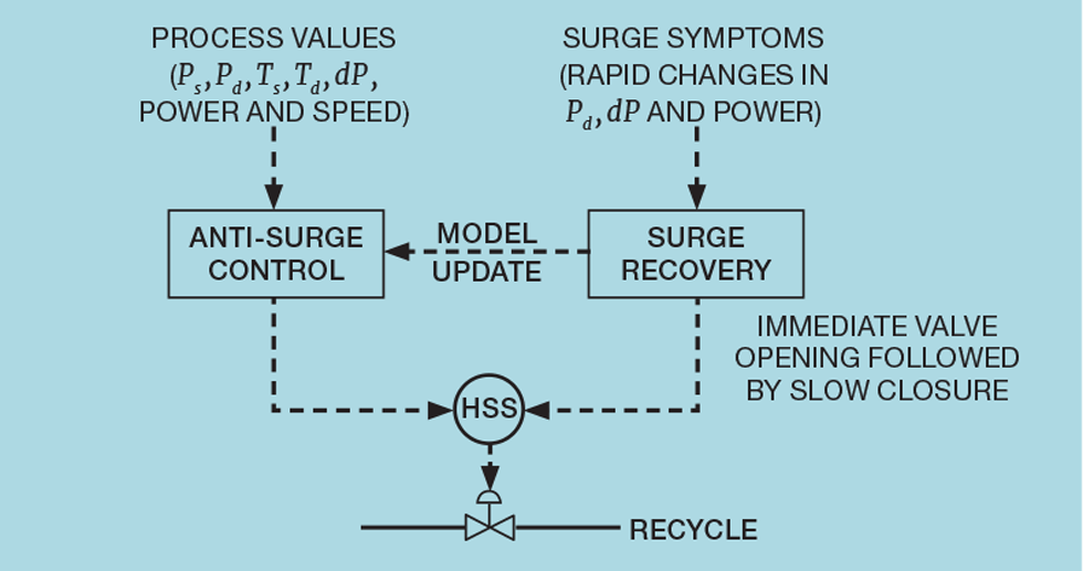
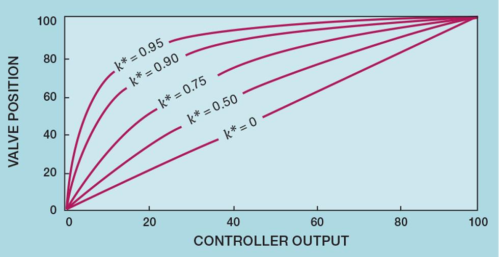
It is common that the recycle valve is a quick-opening type. Like the equal percentage valve, this is achieved by the choice of valve trim or, as shown by Figure 7, by conditioning the controller output (M) to give the valve position (V):

The non-linear behaviour introduced must then be considered when tuning the anti-surge controller.

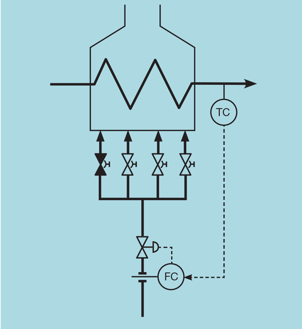
Multi-stage machines

It is common to install multi-stage machines to deliver the required pressure at high flow rates. These comprise several compressors on the same drive shaft. Each will have its own antisurge recycle. Opening the recycle on the first stage will reduce the flow to the subsequent stages, potentially taking them into surge. This can be pre-empted by feedforward schemes that simultaneously adjust all the recycles.

Parallel compressors

It is similarly common, to deliver the necessary gas flow, to install compressors in parallel. Even if purchased as “identical” machines, their performance curves will be slightly different. The problem that can arise is illustrated in Figure 8.

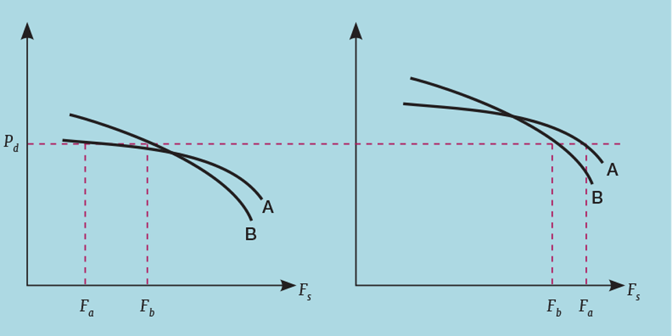
Since they will have the same discharge pressure there will be a difference in the flow through each. The curves on the left of the figure show the flow through compressor A is less than that through B. However, a small change in a suction parameter, such as an increase in molecular weight, will cause the curves to move. In this example the flow through compressor A changes from close to surge to close to stonewall. To avoid reaching such limits, the flows are balanced by employing the scheme shown in Figure 9.

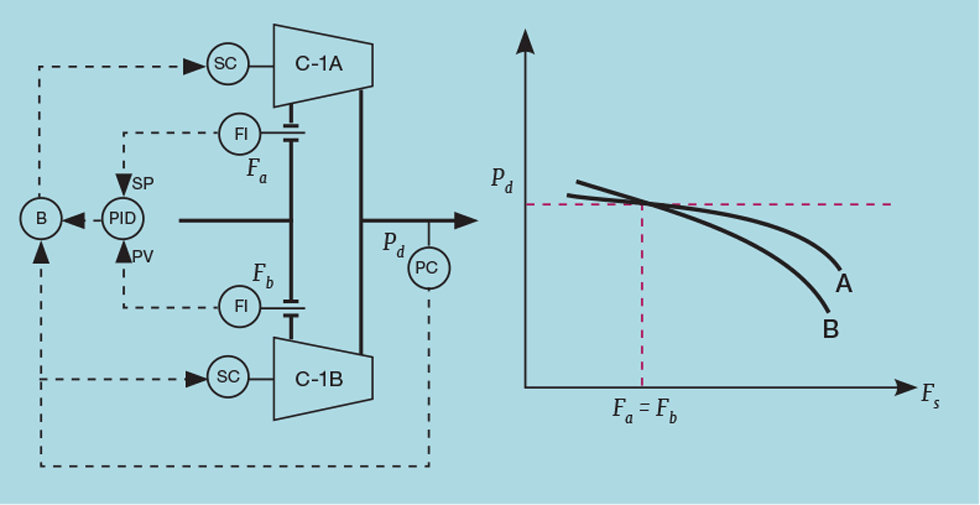
In this example, discharge pressure is controlled by adjusting speed. The difference in speeds is the bias (B), which is adjusted by a PID controller to keep the two flows equal.

---

Myke King CEng FIChemE is director of Whitehouse Consulting, an independent advisor covering all aspects of process control. The topics featured in this series are covered in greater detail in his book Process Control – A Practical Approach, published by Wiley in 2016

---

Disclaimer: This article is provided for guidance alone. Expert engineering advice should be sought before application.