Practical Process Control Part 13: Signal Conditioning

Myke King shows how signal conditioning can resolve non-linearities

CONTROL engineers prefer linear processes. Taking flow control as an example, they like to see a linear relationship between the measured flow (f) and the control valve position (v). A constant process gain, K_p (the slope of this relationship) means the correctly chosen controller gain (K_c) will work over the whole operating range.

Flowmeter

The most commonly installed flowmeter is the orifice type. Pressure drop (dp) across the orifice plate varies with the flow and so flow can be determined by measuring dp – according to:

c_d is the discharge coefficient (typically between 0.6 and 0.8), d the diameter of the orifice and ρ the fluid density.

The pressure drop is transmitted to the control system, but it is the square root of this value which is used by the controller. Known as square root extraction, it is an example of signal conditioning applied to achieve linearisation.

Equal percentage

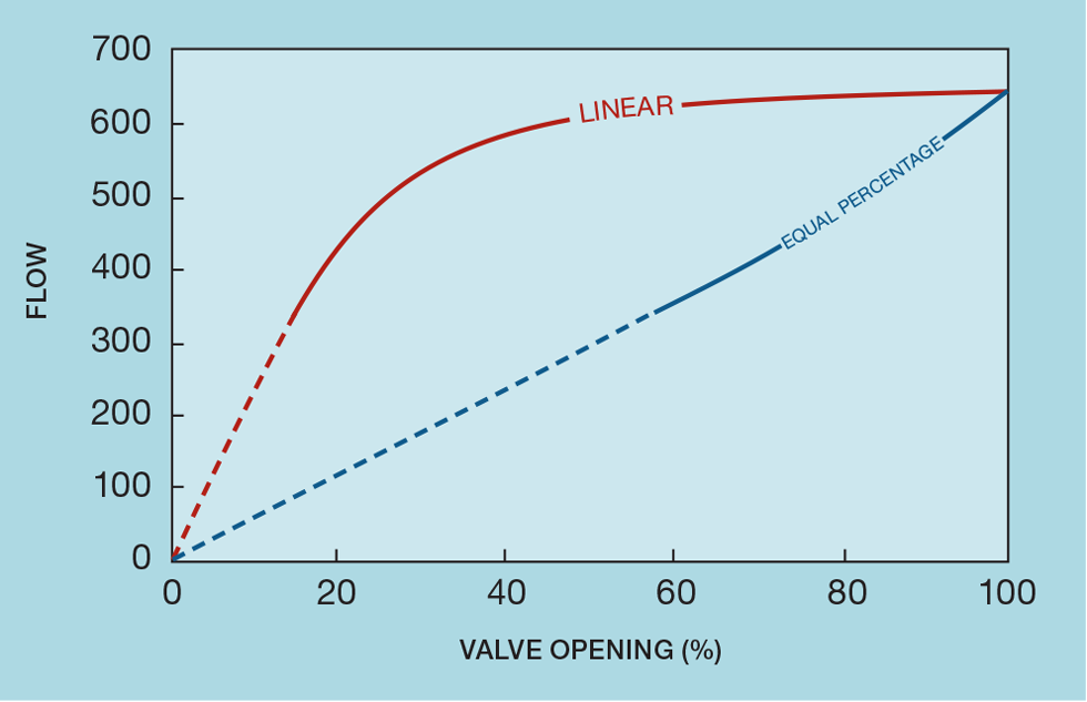
Despite its name, the installation of a linear control valve does not generally result in linear process behaviour. A commonly installed alternative is the equal percentage valve. Figure 1 shows its principle; a given increase in valve opening will result in the same percentage increase in flow. 

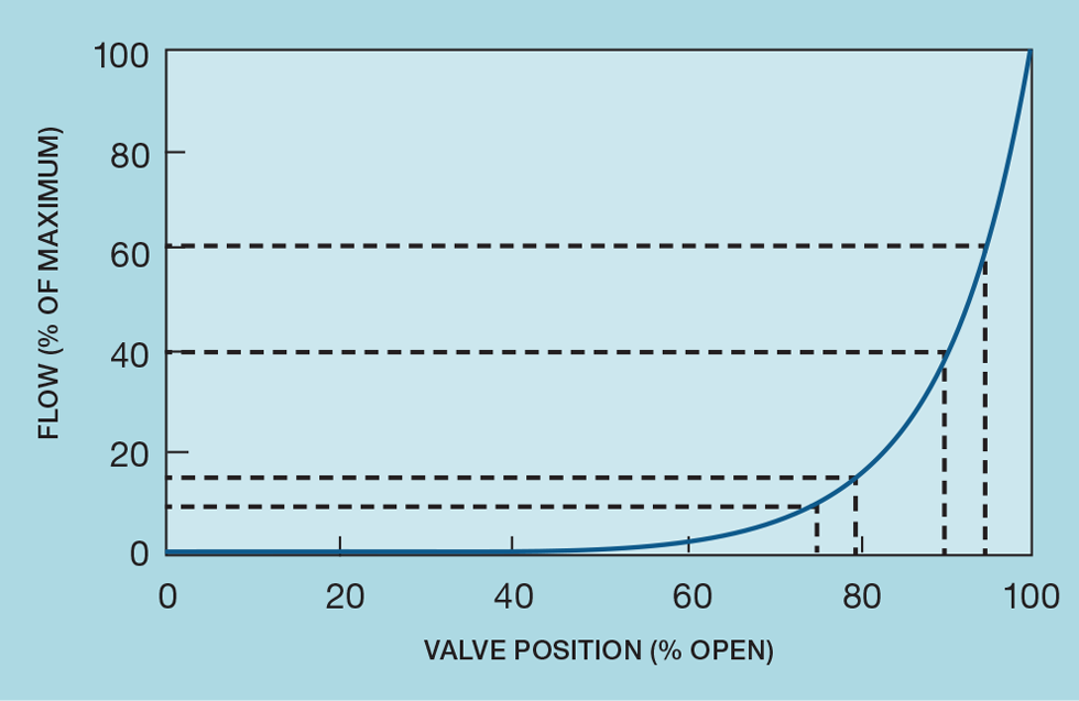
For example, the change in valve opening required to increase the flow by 50% (from 40 to 60) is that same as that required to increase the flow from 10 to 15. The increase in flow from f₁ to f₂, resulting from increasing the valve position from v₁ to v_2, is governed by:

(where k is the valve constant)

Integrating introduces the constant A:

To eliminate A we define F as the flow through the valve when 100% open:

And so:

Note that this equation fails in that it does not give zero flow when the valve is fully closed (v = 0). So, in practice, equal percentage valves do not exactly follow the theory.

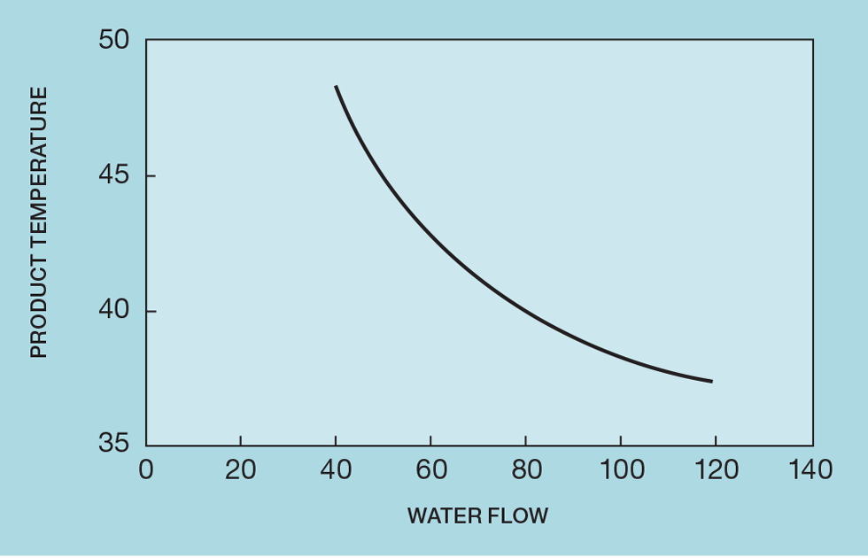
Product cooler

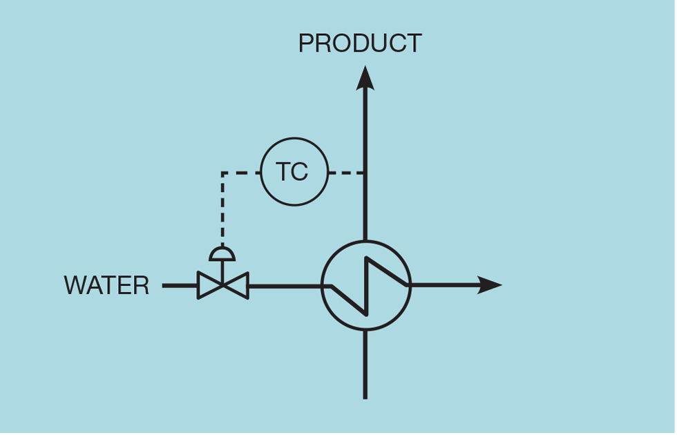
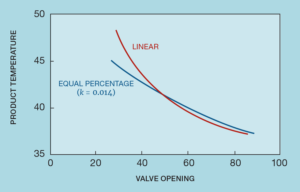
Figure 2 shows a commonly installed scheme, in this case manipulating cooling water to control product temperature. Figure 3 shows how this temperature varies with the flow of water. Since it is unusual to install a flowmeter on the water supply, the curve is derived from heat exchange equations, rather than collected data. As might be expected, the result is non-linear. Horizontally, the curve is asymptotic to the temperature of the cooling water. However, what is of interest for controller tuning is the relationship between temperature and valve position. As Figure 4 shows, if we were to install a linear valve, the slope of this relationship varies over the operating range (by a factor of around five). This would cause severe controller tuning problems. The choice of an appropriate equal percentage valve almost linearises the relationship.

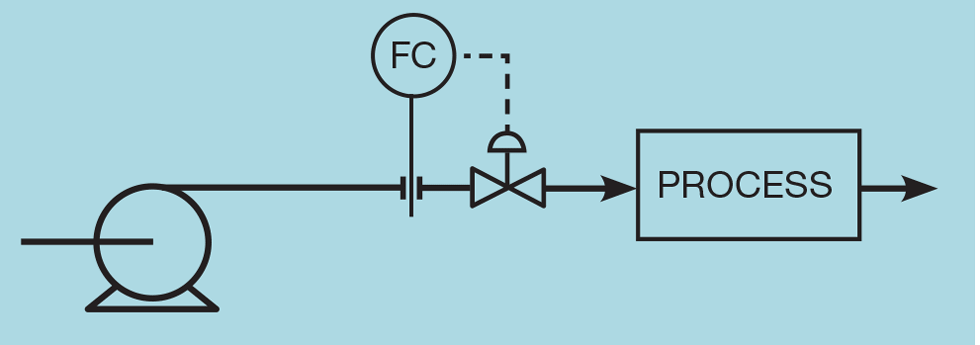
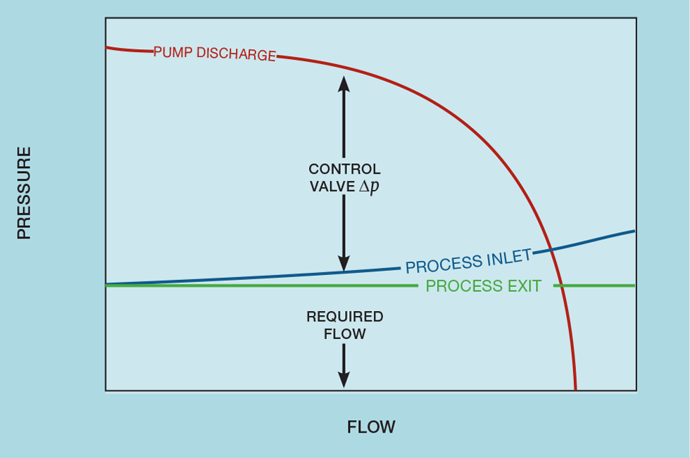
Pump flow control

Figure 5 shows a typical pump flow controller. Figure 6 shows how pressures in the process vary with flow. We assume that the product is routed to storage, so that process exit pressure is constant. As with our orifice plate, the pressure drop through the process is proportional to the square of the flow. The process inlet pressure is therefore a quadratic function. The figure also shows the pump performance curve. In the absence of the control valve, the process will operate where the pump curve intersects the process inlet curve. The inclusion of the valve generates a pressure drop. By adjusting the valve position we change the pressure drop and so the flow. However, the pressure drop is the difference between the two curves and so varies in a highly non-linear way. Figure 7 shows the behaviour of a flow controller manipulating a linear valve (plotted from plant data, the dotted line shows extrapolation below the minimum flow of 340). Use of an equal percentage valve (with k = 0.015) almost exactly linearises the process.

The chart also shows why instrument engineers will often specify equal percentage valves in situations not necessarily justifying their use. In this example the valve travel is about half of that of the linear valve. It can thus operate over a wider flow range and so will be more forgiving of any sizing error.

Output conditioning

While conventionally a control valve type is chosen so that process behaves linearly, non-linear compensation can alternatively be included in the control system. Known as output conditioning, this comprises some simple calculation applied to the controller output (M) before it is transmitted to the valve positioner.

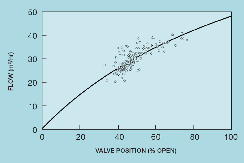
As we saw in TCE 987, the relationship between flow and valve position can be described by:

(where k is a valve constant but defined differently to that in the equal percentage characterisation).

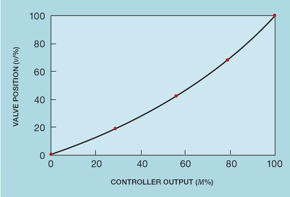
Figure 8 shows the process data used in TCE 987. Curve fitting gives F as 48.2 and k as 0.43.

By differentiating we can obtain the process gain:

As v varies from 0 to 100%, the process gain therefore varies over the range:

For the process to be treated as linear, the process gain should vary by no more than ±20%. So, the maximum gain should be no more than 1.5 times the minimum:

If operated over the whole range, our flow controller substantially exceeds this value. But the data show that, for normal operation, the valve position varies between 30 and 80%. The process gain therefore varies between 0.33 and 0.56 – still outside our tolerance for linearity.

To apply output conditioning we simply invert the valve curve (as shown in Figure 9), so:

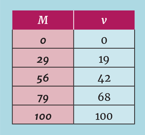
Some control systems support such a calculation being applied to the controller output. Others permit a look-up table, typically containing five values. The first and last entries of this table must be 0 and 100%. Table 1 shows the values chosen so that four straight line segments closely match the curve.

Gain scheduling

While both conditioning approaches work well, they suffer the disadvantage that the displayed controller output will be different from the actual valve position. While we can train operators to understand this difference, a more elegant approach is to change the controller gain as operating conditions change. This is known as gain scheduling. We know that K_c is inversely proportional to K_p. So, from above:

To apply this, we determine the controller gain (K_c*) at a typical valve position (v*). Then, as the valve position changes, we adjust the controller gain according to:

So, in our example, we might choose 50% as the typical position. As the valve moves from 30 to 80%, the controller gain would be changed from 0.79K_c* to 1.36K_c* As with output conditioning, depending on the control system features, this might be implemented as a calculation or as a look-up table.

Constraint conditioning

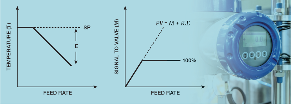
Figure 10 shows a simplified example of the application of multivariable predictive control (MPC). Such strategies capture the bulk of the benefits of improved control. They do so by more closely approaching operating constraints. Our example shows the controller manipulating the setpoint of the feed flow controller in order to fully utilise capacity. One of limiting constraints is a hydraulic limit on the fuel supply to the fired heater. The output of the fuel flow controller (M) tells us how closely this limit is being approached. Ideally, we’d like to permit the control valve to operate at 100% open, but this would mean losing control of the temperature. For example, if a process disturbance causes the temperature to fall below its setpoint, the controller could do nothing to correct this and the MPC will not make the necessary reduction to feed rate. The operator would therefore typically set a limit of around 90% – sacrificing some capacity.

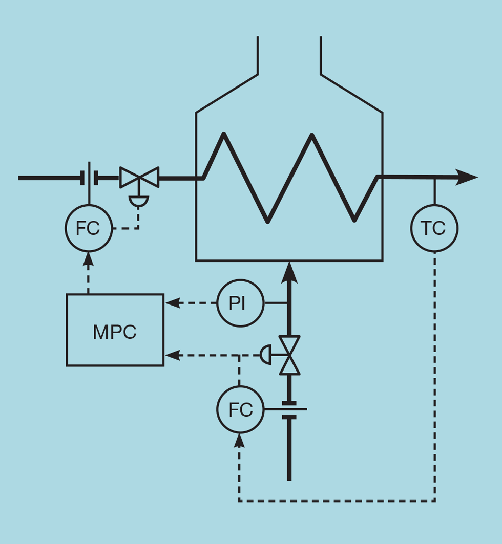
Constraint conditioning resolves this limitation. In this example, if the feed rate exceeds capacity, the heater outlet temperature will fall below setpoint. We can condition M using the controller error (E) – as shown in Figure 11. This virtual valve position (PV) can now exceed 100% - allowing the operator to safely increase the maximum closer to 100%. For the behaviour of the virtual valve to follow a linear extrapolation of the real valve, we set K to the process gain between valve opening and temperature (obtained when operating just below capacity).

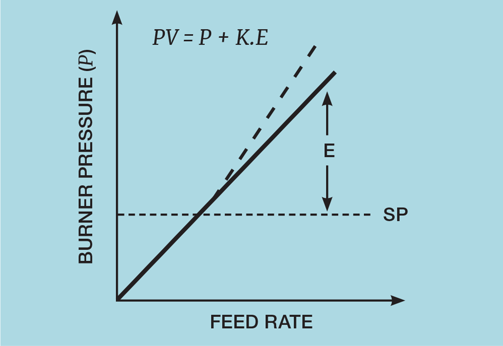
Another form of conditioning can be applied in situations where we want a non-symmetric response to approaching a constraint. The second constraint included in Figure 10 is the maximum burner pressure. Unlike the fuel valve position, which is a hard constraint, burner pressure is a soft constraint. While undesirable, the constraint can be approached from either side. But we want violation of the constraint to be resolved more quickly than approaching it from below the limit. Figure 12 shows how this is achieved. If the burner pressure is above the limit (E > 0), the MPC “thinks” the pressure is higher than it actually is and so takes faster action. But care needs to be taken; too high a value of K will cause the MPC to go unstable. Typically it should be below 0.2.

---

The topics featured in this series are covered in greater detail in Myke King's book, Process Control – A Practical Approach, published by Wiley in 2016.

---

This is the thirteenth in a series that provides practical process control advice on how to bolster your processes. To read more, visit the series hub at https://www.thechemicalengineer.com/tags/practical-process-control/

---

Disclaimer: This article is provided for guidance alone. Expert engineering advice should be sought before application.