Modelling with Excel Part 6: Monte Carlo Simulations

Stephen Hall continues his series on how to use Excel for project engineering. Download the interactive workbook to experiment with as the series develops

People often ask me if my simulations include a “Monte Carlo” analysis. Why not “Las Vegas” or “Macau”? These are places that I associate with gambling, and what these people are asking is whether my simulations are stochastic by considering randomisation or a “roll of the dice.”

Atomic secrets

The answer to “why Monte Carlo?” - unlikely though it may seem - lies in the desert of New Mexico in the 1940s. As part of the Manhattan Project, the allies’ effort to develop an atomic bomb, Hungarian-born physicist Stanislaw Ulam needed to model the diffusion of neutrons though a mass of uranium undergoing nuclear fission. This couldn’t be achieved using then-available calculation techniques, because of randomness induced by neutron collisions with nuclei. While ill and killing time playing Solitaire, Ulam tried to calculate the likelihood of winning. Realising this could be the key to the neutron problem, he joined forces with his countryman, mathematician John von Neumann, and used his card-playing insights to develop a mathematical method for taking account of randomness. As everything to do with the Manhattan Project was top secret, Ulam and von Neumann needed a code-name to refer to their method in reports, and inspired by the connection with cards, and the fact that Ulam had an uncle who was a compulsive gambler at the Monte Carlo Casino in Monaco, it became the Monte Carlo method and remains so to this day. Chemical and industrial processes are rife with uncertainty and unplanned events. Shouldn’t our models be similarly dynamic?

Stochastic simulations incorporate randomisation for many reasons. One of the main reasons is to account for variability in the model parameters and initial conditions. Randomness helps to generate a range of possible outcomes, reflecting the true nature of complex systems. By incorporating randomisation, stochastic simulations can provide more realistic and accurate predictions of system behavior than deterministic models, which do not incorporate randomness. Another reason to use randomisation in stochastic simulations is to explore the effects of different scenarios and interventions. By simulating a range of possible outcomes, one can evaluate the impact of different factors and interventions on the system’s behaviour and identify optimal design or operational strategies. Overall, stochastic simulations are a powerful tool for modelling complex systems and generating insights into their behaviour.

Relating randomness to modelling

There are three broad categories of simulations. Continuous processes run at a “steady state” but produce output that may fluctuate over time. Randomisation in continuous modelling can introduce perturbances such as flow or concentration changes, which can shed light on how the system will react to these varying conditions. If the model includes a simulated process controller, its proportional integral derivative (PID, see process control articles) parameters could be adjusted to predict the controller’s behaviour. That was the purpose of the wastewater neutralisation model that is briefly described in the introduction to this series (Issue 980, February, 2023).

Batch processes take a fixed quantity of material and transform it in some manner. In this type of simulation, randomisation is applied to the quantities of starting materials, time to start or end a batch (batch starts and ends are often performed manually), and the duration of the batch. These models show the different steps of a batch along a timeline that is often visualised with Gantt charts (Issue 984, June, 2023). For example, the simulation could establish a batch starting time as the start of the operator’s workday but then randomise a time delay to account for things like staff meetings and coffee breaks. There may also be randomised stoppages or delays for equipment issues or quality checks.

Discrete models count occurrences when a process is divided into individual events or steps. Goals for the simulation include determining how many of an item, such as an intermediate bulk container, are in use, or estimating the maximum wait times at certain steps in the process. For example, people need to don gowns before entering a pharmaceutical or microelectronics cleanroom. Using their arrival times, time to put on the gowning, and capacity of the gowning room, the overall time to assemble the full complement of operating staff can be calculated. Randomisation can be assigned to the time variables, which gives a more accurate and complete picture when the simulation is repeated many times compared to the initial static calculation that is based on a single set of input assumptions. This information is valuable for identifying bottlenecks, optimising process flow, and improving overall system performance.

Chemical and industrial processes are rife with uncertainty and unplanned events. Shouldn’t our models be similarly dynamic?

Distributions and statistics

In a model, each randomised variable will typically change with every iteration. For instance, in a fermentation process, the time required to reach the desired cell density is subject to many variables. These include the initial number of bacteria in the seed broth, the quantity of carbohydrates in the media, and the growth conditions, including pH, temperature, and air flow rate. A model that incorporates these factors to calculate cell growth may randomise the values of the factors to generate a range of possible fermentation times. Running this model several times allows for an estimation of the distribution of fermentation times that could occur under different conditions, providing insight into the best strategies for managing the fermentation process.

The values for the randomised variables are obtained from a continuous or a discrete distribution. Continuous distributions follow probability distribution curves such as Normal, Exponential, Weibull, etc. If you have data from an existing process, you can find the distribution that fits it best and use the fitting coefficients in your model. For example, with a normal distribution your coefficients are the mean and standard deviation for the observed data. For a new process or one for which you do not have reliable data, you can choose a distribution that is usually used for that type of variable and make educated guesses for the coefficients; you can test different coefficients to perform a sensitivity analysis and assess the importance of fine tuning your guesses.

Discrete distributions assign probability to each of several possible values for the variable. The distribution might resemble a continuous distribution in the sense that a mass plot of the values may have a shape that is similar to, for instance, a bell-shaped normal distribution. For example, your model might limit possible batch sizes to five volumes, each with a probability. If the sizes are spaced around the middle, with the middle of the five having the highest probability, the mass curve will look like a normal distribution, even though it is a discrete distribution.

But a discrete distribution could instead have no discernible relationship to a continuous distribution. A second variable for example might be the solvent that is used in a batch. Four different solvents, with probabilities (summing to 1) for which a statistical distribution has no meaning.

Obtaining the random input from a distribution

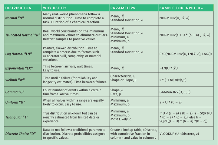
In Excel, you can generate the randomised inputs from a continuous or discrete distribution using worksheet formulae or VBA subroutines with a technique that is called “inverse transform sampling.” Excel has built-in inverse functions for the distributions listed in Table 1. The formulae take a random number, U, from 0 to 1 and “transform” it into a value that falls onto the distribution’s continuum.

For example, if your simulation includes the time to complete a chemical reaction in a batch reactor, you can model the time using a normal distribution. From data or experience, find the mean and standard deviation for the reaction duration. Each run of your simulation assigns the reaction time by generating a random number and applying the Normal distribution formula from Table 1.

Visualisation

I find it useful to create charts for the distributions before I use them in a model. This lets me fine-tune the parameters, or change the type of distribution, and see the effect on the range and variability of the randomised input. The histogram (Figure 1) shows the number of samples that fall into ranges. A line chart (Figure 2) sequentially pulls 100 random numbers and shows how the random sample bounces up and down. This chart is especially useful in highlighting the frequency and extent of outliers.

Generating the random samples

To obtain the random inputs, a random number from 0 to 1 is needed. This can be placed into a cell or embedded in the formulas from Table 1.

As seen in the downloadable companion workbook (https://bit.ly/ModellingWithExcel), Excel’s random number generator, RAND(), updates every time any cell in the workbook is changed. This may be undesirable because the results that are computed and displayed will constantly change, but you might want them to remain static until you purposely update the random numbers. Visual BASIC for Applications (VBA) can help. By identifying the cells and ranges that contain a random number, you can create a VBA subroutine that repopulates them on command. In other words, generate the random number in a VBA subroutine and have the subroutine write the answer into the worksheet cell instead of using the RAND() formula in that cell. The number, and results that are based on it, will remain unchanged until the subroutine is executed again.

Instead of generating random numbers in VBA and copying them to the worksheet, the entire inverse sampling method can be performed within VBA with the resulting random sample saved to the worksheet. The advantage of this approach is that the type of distribution is easily changed without having to edit any formulae; only the input values would be modified.

Listing 1 gives my generalised solution as a VBA User-Defined Function (UDF). The function takes two arguments. The first argument is a code letter (or letters) that define the distribution to use, followed by the parameters that the distribution requires with a “/” to delimit these elements. For example, “N/14/2” means, “use a normal distribution with mean 14 and standard deviation 2”. If you use this UDF on a worksheet, by including RAND() for the second argument the resulting random sample will change whenever any cell is changed on the worksheet. The second argument is optional, however, and if it is omitted the result will only change if the input string for the first argument is changed. The beauty of this solution is that an input’s distribution function is changed simply by modifying the input argument; no formulae need to be updated. This UDF can also be called by another subroutine which is handy when a simulation is managed by VBA routines.

Another advantage of VBA is that you can create a sequence of random numbers that is the same every time that you run the subroutine. This lets you test your simulation with the exact same randomness before running it with a fully random set of inputs which can be helpful as the model is being debugged and optimised.

VBA has the RND(x) function for generating random numbers. If “x” is a negative number, it acts as a seed for the random number generator and initiates a sequence of numbers that can be repeated if the same seed is used again. If “x” is 0 or a positive number, the function continues the sequence of random numbers started by the seed. However, if “x” is omitted, as in RND(), a new sequence is initiated using an internally generated seed value. In contrast, the worksheet function RAND() does not offer this level of control; it generates an unpredictable random number each time it is used.

Summary

To execute a Monte Carlo simulation, selected inputs are randomised and the simulation is run many times with results collected and analysed. Over many trials, the value of the randomised input can follow one of many possible statistical distributions. This helps analyse the impact of input variations on the process or the simulation outcomes., and it can help establish the design space for the process. Table 1 provides commonly used distributions as input assumptions for the Monte Carlo simulation. However, when sufficient real-world data is available, a statistician can analyse the data to determine the best-fitting distribution.

The companion workbook demonstrates the use of formulae for sampling each of the distributions. From a random number, a value from the distribution is determined. The values that are returned from a large number of such samples will follow the specified distribution, but each sample could be any value in the possible range that the distribution defines. This is why many runs of the simulation are needed before drawing conclusions.

This is the sixth in a series that provides practical guidance on using Excel for project engineering. Download the companion workbook from https://bit.ly/ModellingWithExcel

To read the rest of the articles in this series, visit the series hub at:  https://www.thechemicalengineer.com/tags/modelling-with-excel

---

Disclaimer: This article is provided for guidance alone. Expert engineering advice should be sought before application.