Modelling with Excel Part 7: A Comparative Study ‑ Part 1

Stephen Hall continues his series on how to use Excel for project engineering. Download the interactive workbook to experiment with as the series develops

THIS month and next I will show a variety of ways to model a batch process. Excel is a blank canvas that provides immense flexibility with a model’s design. I will illustrate simple and complex ways to approach my example problem and discuss their strengths and challenges. The articles present several solutions to the problem. They use the Gantt chart and Monte Carlo tools that I provided in Issues 984 and 985/986, and provide some more tips and tricks along the way.

Problem statement

Consider the Central Services department in a facility, where many automated single-door washers are used to clean parts from the facility’s manufacturing lines. How many wash loads can be completed in a day, given a specified number of washers and washing recipes? What changes when random delays between loads are introduced that represent staffing conflicts or equipment problems? Is it worthwhile to provide operating crews for loading and unloading multiple washers simultaneously?

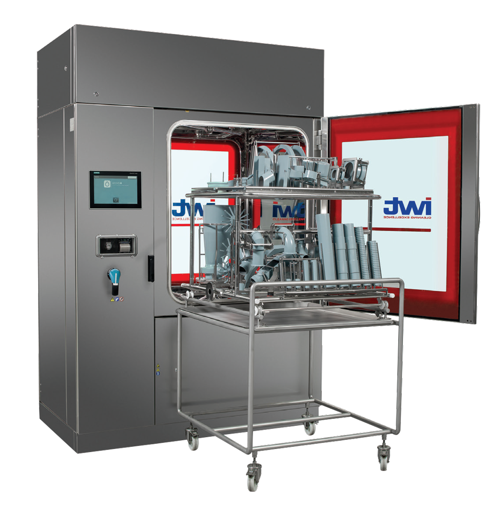
A typical parts washer is shown in Figure 1. This one has loading and unloading doors on opposite sides, but my example stipulates that there is only one door with loading and unloading from the same side. Manufacturing personnel deliver soiled parts to Central Services. The operators in Central Services arrange the parts on racks in prescribed load patterns, roll the racks into a washer, select a washing recipe, and press the “Start” button. When the load is washed and dried, the washer signals completion. The operators remove the racks from the washer and transfer the cleaned parts to bins, carts or trolleys; they often cover the cleaned parts with plastic before discharging them back to Manufacturing for storage or use.

Excel is a blank canvas that provides immense flexibility with a model’s design. I will illustrate simple and complex ways to approach my example problem and discuss their strengths and challenges

Inputs

Before analysing the operation, wash recipes must be specified. On the companion spreadsheet you will find that the Inputs for this exercise are consolidated as seen in Figure 2. There are three possible recipes that define the durations for 11 steps. The water recirculation and final rinse steps may be repeated as defined in the recipes. Each of the durations can be set definitively or stochastically using the codes that I presented in Issue 985/986. The calculations presented in this article randomise the manual steps (load and unload) and the recirculation and rinse steps. You can change any of the inputs and run new calculations to test different scenarios.

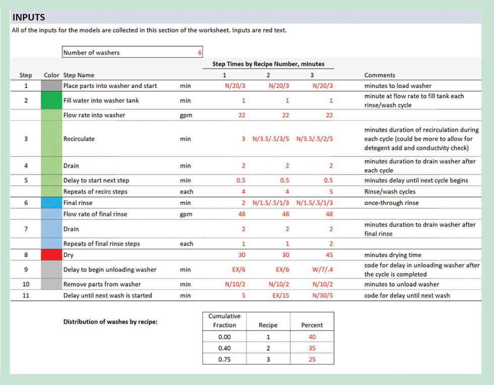
The number of washers in the washroom and the distribution of wash loads among the three recipes are also specified in the Inputs section. This completes the data input for the project.

The Excel worksheet for this month includes five calculations; I will discuss four more next month. I created a summary section (Figure 3) near the top of the sheet to ease comparisons between their results. I describe each of the calculations in the next section.

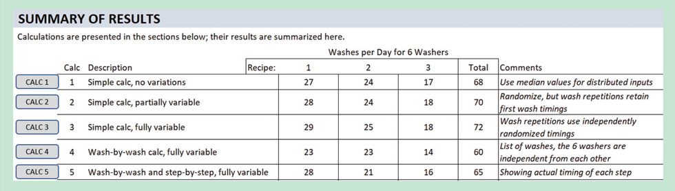
The calculation methods are increasingly complex. However, the answer to the basic question, how many loads per day, does not differ significantly if resource levelling is omitted. With complexity comes added time to develop and debug the calculations. The primary message I want to convey is this: Excel is a powerful tool that I am passionate about using. But it is easy to get mired in excessive detail and complexity. Take time to define the goals carefully before plunging into a comprehensive modeling exercise. You might find that a very simple approach will provide the answers that you seek. Be sure that your source data – the model’s inputs – are sufficient to produce the desired results. Look for simplifications. And obsessively test the results.

The calculations

In keeping with my approach to previous articles in this series, I want readers to follow my thought process as I worked through the five calculations that I prepared to answer the problem challenge. I decided to hard-code the models to use the 11 recipe steps shown in Figure 2 and limit the number of recipes to three. I used the “TestDist” worksheet to visualise the randomised recipe entries. I also decided to do the calculations against a 24-hour day. Finally, I am only counting wash loads that are completed within the single day of the exercise; spillover to the next simulated day eliminates a load from the count.

Calc 1 simply adds up the time for the 11 steps, with multipliers for the wash and rinse steps that can be repeated. For the randomised inputs I assigned a “random” number of 0.5 which gives the median value, not the average, for those inputs. Although the calculation can be entered into one long formula on the worksheet, I implemented it in a User Defined Function (UDF) to make it easier to write and debug. After I decided how I was going to do this calculation, it took me about ten minutes to write and enter the UDF.

The results from Calc 1 are given as the time to complete one load and the number of loads per day per recipe. I needed a second calculation to assign the recipes according to the recipe distribution table to arrive at the total number of wash loads per day.

I used an iterative approach for this. To get the final answer, I wrote a subroutine that starts with a guess for the number of batches that use Recipe 1. From the recipe table, it calculates the batches for Recipes 2 and 3. It totals the time for all three recipes and compares this to the time that is available in a day (i.e., number of washers x minutes per day). The initial guess is purposely high so the calculated time exceeds the available time. The algorithm decreaces the number of Recipe 1 batches by one and repeats the calculation, continuing in this loop until the calculated time is less than the available time.

Calc 2 is like Calc 1, but instead of fixing the times for stochastic variables, it randomises each of them. In the steps that are repeated (wash and rinse), the same value is used for all loads. Calc 3 takes this one step further and randomises the repeated steps, so if there are three rinses they will each have a different duration.

I applied the same iterative subroutine for determining the total loads according to the recipe table for Calcs 1 through 3. Clicking on the “Calc 1”, “Calc 2”, and “Calc 3” buttons (Figure 2) updates the estimates. Since Calc 1 uses the median value for the stochastic inputs the answer doesn’t change. All three calculations derive the duration of just one load for each recipe and uses that duration for all of the loads in the day. Therefore, they are not fully random. The next calculation remedies that shortcoming.

Beyond simplification

The remaining calculations (some will be discussed in the next issue) randomise every step in every load and perform load-by-load time summations until the simulated day is complete. Each load is randomly assigned a recipe according to the recipe frequency table. Unlike the preceding calculations, the distribution of loads for a single simulated day might not exactly match the recipe table. This is a realistic outcome of using a Monte Carlo method; over many simulated days the accumulated recipe distributions will match the table.

The results are tabulated in the respective sections of the worksheet. The length of these sections changes with each iteration of the calculations, especially if the number of washers changes. The subroutines dynamically adjust the number of worksheet rows for the calculation sections. Examine the VBA code in the companion workbook to see how.

Calc 4 uses a subroutine that is very similar to Calc 3 to fully randomise each simulated load. To provide some additional information, the subroutine tabulates the time of day for each load’s start and finish. The calculation is initiated by clicking the “Calc 4” button, and by repeatedly running it you can get a sense of the range of answers. It took me a little longer to program this compared with Calcs 1-3; the results are the same, however, and the added value is limited to the load-by-load tabular results table which gives some insight as to how the loads are spread out over the day.

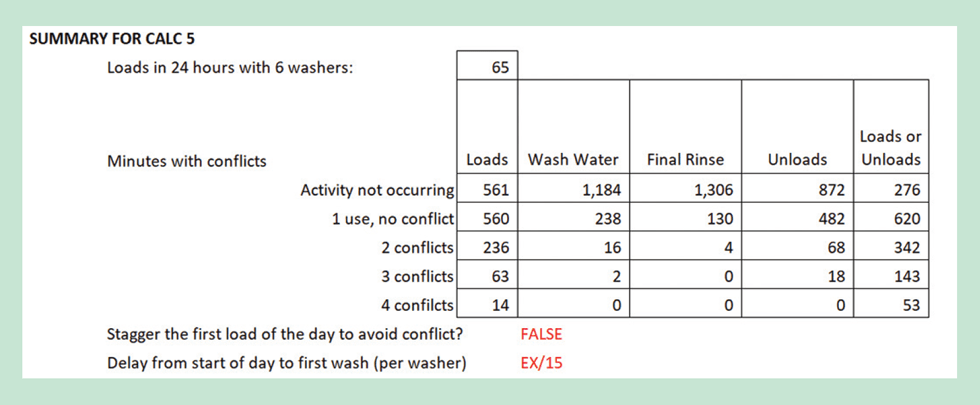
Calc 5 layers in the full timeline for each load. In addition to the load-by-load tabular results, Calc 5 provides a minute-by-minute accounting for each wash load. Because the water rinse steps can be as short as 1 minute, I divided the day into ½-minute intervals and created a matrix with 2,880 columns (the number of minutes in a day multiplied by 2) and rows equal to the number of loads. The calculation counts when there are simultaneous occurrences of the manual loading and unloading operations, and simultaneous water draws as shown in Figure 4.

The timing matrix provides the information needed to create a Gantt chart visualisation. After setting up the Gantt chart using the routines given in Issue 984, a subroutine uses the matrix to determine where to place the activity bars for each washer, grabbing colours from the Inputs section of the worksheet. I reduced the fidelity of the Gantt chart to show only the Loading, Washing, Drying, and Unloading phases, eschewing the fine details of the recipes, because this is enough to tell the story. See the next issue for an illustration of the Gantt chart.

The complexities of these calculations - some of which will be fully discussed next issue - meant that designing, writing and debugging the algorithms took me many hours. I wanted to implement the solutions on the worksheet to help me visualise answers, debug the code, and easily use the data for making the Gantt chart. On my first attempt, calculation 7 - which manipulates the result of Calc 5, discussed above - took more than five minutes for a six-washer case. I added timers to help me find better approaches. This execution now completes in less than 15 seconds. This is still lengthy, and in the next issue (as well as discussing Calcs 6 and 7) I will show how to reduce this to a fraction of a second.

The lesson, though, is that complicated does not necessarily equate to “better”. It depends on how the results will be used

Lessons learned

Each of the five calculations presented in this article estimate the number of wash loads for a single day. With each iteration the calculations are more sophisticated in the sense of how they treat the stochastic variables and present the results. But they do not resolve conflicts, such as simultaneous draws from the water system. They also fail to deliver on a Monte Carlo’s core objective of evaluating the effects of variations over time.

Despite the increased complexity of the calculations, the results are comparable; the simplest Calc 1 is just as valid as Calc 5 for estimating the total number of loads that can be processed in one day. To get a quick sense of the variability over time, click repeatedly on the respective calculation buttons for Calcs 2 or 3 on the worksheet. Simply observing the total loads per day result over many recalculations gives the answer. This might be sufficient to meet the objective of the calculation and the total time to develop the worksheet could have been a few hours.

For presentation purposes or to support a written report, it may be worth the significantly added effort to program the load-by-load details that Calcs 4 and 5 provide. The lesson, though, is that complicated does not necessarily equate to “better”. It depends on how the results will be used.

This is the seventh in a series that provides practical guidance on using Excel for project engineering. Download the companion workbook from https://bit.ly/ModellingWithExcel

To read the rest of the articles in this series, visit the series hub at:  https://www.thechemicalengineer.com/tags/modelling-with-excel

---

Disclaimer: This article is provided for guidance alone. Expert engineering advice should be sought before application.