Modelling with Excel Part 4: Batch Heating and Cooling

Stephen Hall continues his series on how to use Excel for project engineering. Download the interactive workbook to experiment with as the series develops

This article walks through the creation of a model for heat transfer in a jacketed tank, tracking performance over time, to construct cooling and heating curves. This is an example of a batch process where a fixed quantity of material is processed as a unit. The simulation calculates the time to complete the batch (in this case, the time to reach a target temperature) and the resources that are required to process it (energy in this example).

There are two goals for this model. 1) Predict the heating and cooling times for a small mixing vessel along with the heating and cooling duties, and 2) Show how the times are affected when the jacket fluid is changed, or its temperature or flow rate are adjusted. Tank heating or cooling calculations require knowledge of the heat transfer coefficients and thermodynamic properties of the fluids. I am constructing this model with simplifications; additional details can be added later.

One learning objective is to understand the stepwise organisation in the workbook that calculates the changing heat transfer at user-designated time intervals. Another is to use dynamic naming to establish the data parameters for charting the results. We will employ the tools that I described in the first three installments of this series (Issues 980, 981, 982). The completed model is available for download from https://bit.ly/ModellingWithExcel

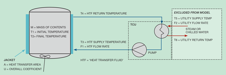
The flow diagram for the model is given in Figure 1. Ignore the building utilities (F2, T5, and T6) by assuming that the temperature control unit (TCU) has capacity to maintain a constant temperature for the heat transfer fluid (HTF). The other parameters shown on the diagram are either specified by the user or calculated by the model. For heating, T3 > T1; for cooling, T3 < T1. T3 can either be fixed (T3 = constant) or controlled to keep it at a certain value above (or below for cooling) the tank temperature (e.g., T3 = T1 + 10).

The general approach for the model is to define parameters for Figure 1 at the beginning of the heating or cooling cycle, calculate the heat flux through the jacket for those conditions, apply that heat to the material that is inside the tank, and determine a new set of parameters after the designated time increment. The procedure will be repeated until the temperature target is reached.

Heat transfer coefficients

Heat transfer is calculated with Equation 1. The key parameter is U, the overall heat transfer coefficient. Representative values of U are tabulated for common tank configurations in reference books. I am going to choose to start with a value of 750 W/m²-K and assert that this is representative for a jacketed tank with water at 20°C in the jacket but make this a user input to facilitate a sensitivity analysis. We know, however, that U changes with the properties of the fluids, especially viscosity. Since the model’s goals include comparing heat transfer for different HTFs, adjustments to the initial U must be incorporated into the calculations. I will do this by creating a calculation for the outside film coefficient, which changes with the properties of the heat transfer fluid, as explained in the following paragraphs.

Several resistances to heat transfer are combined to compute the overall coefficient per Equation 2. The fouling (fj, fv) and wall resistances (x/k) are usually small compared to the inside and outside film coefficients, hi and ho.

Simplify the problem by keeping the resistances and inside coefficient constant. Then focus on the effect of the jacket fluid properties. Therefore, assign R to represent the last four terms of Equation 2 to define Equation 3.

It is reasonable to estimate ho by using the relationship for fluid flow inside a pipe. Since the initial U is based on water in the jacket, use the properties of water to compute a baseline ho and from that R. It follows that, since R will be kept constant, changes to the jacket fluid properties can be used to recalculate ho and U for the simulation.

Use the Dittus and Boelter equation (Equation 4) for the Nusselt number to obtain ho, which is valid for turbulent flow. NRe is the Reynolds number, NPr is the Prandtl number (Cp µ / k), Cp is heat capacity, µ is viscosity, k is thermal conductivity, and d is hydraulic diameter.

Setting up the model

Start with the workbook from Issue 982, Physical Properties, that is already configured to deliver physical properties for heat transfer fluids, water, and other substances. Insert a new worksheet. This is going to be a simple model and my plan is to keep all of the inputs, calculations, and output on the single sheet.

Using the rules from Issue 980, immediately give the sheet a title and describe the objective. It would be helpful to include Figure 1 to illustrate the problem although this is not strictly required.

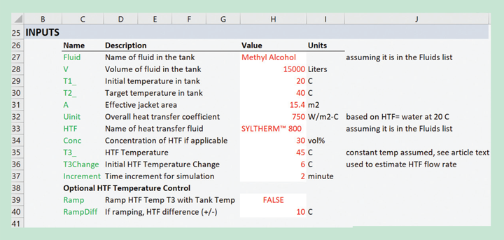
Next, prepare the Inputs area as shown in Figure 2. Name the input cells and populate them with data. While developing a new model you are likely to decide to add new inputs or modify ones that you start with. That is true in this case, and Figure 2 shows the final set of inputs after the remaining steps described here were completed.

Organising the calculation

The next step is to gather any computer-generated parameters, such as physical properties, and perform intermediate calculations. I usually place this immediately below the Inputs section and may consider moving it to another sheet when the model is completed simply to reduce clutter on the main page.

The decision for doing this depends on whether the section is crucial for understanding the flow of the calculation and if a printout of the calculation needs to include the information that is included.

For this model, I want to calculate R from Equation 3. To do that ho is needed, using the assumption that the overall U is based on water in the tank jacket at ambient temperature. We do not know the hydraulic diameter or Reynolds number, so I will assume that the initial U is from a system with d = 0.075 m and NRe is 120,000. Although these are technically user inputs I am placing them in the initial calculations section because I do not want users to change these assumptions. This gives the basis ho as 4030 W/m²-K and R = 0.0011 m²-K/W as seen on the download worksheet.

The second objective of the model is to compare results with different heat transfer fluids. To do this, I am assuming that the velocity through the jacket will remain constant, and different flow rates will be accommodated by proportionally adjusting the number of heat transfer zones within the jacket (which is outside the scope of this model). Therefore, the Reynolds number (DρV/µ) can be calculated for a different HTF or HTF temperature through ρ/µ proportionality. With the new NRe, ho is recalculated and from the assumption of constant R the new U is computed.