Taking a Look Back at Control: Part 2

Martin Pitt considers the history of process control in a two-part series, concluding with electrical and computer systems

IN THE first part of this series, I looked at mechanical and pneumatic controls, with pneumatic control becoming standard in the oil, gas, and chemical industries during the 1940s. Computer systems dominate now but some of the techniques that underpin them owe much to developments which occurred as far back as the 19th century.

Electric devices

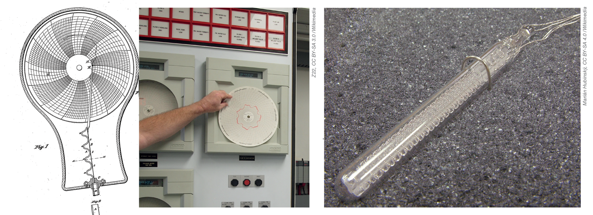
In 1888, William Henry Bristol (1859–1930) patented a “pressure indicator and recorder”, a chart recorder which was to become an essential feature of process plants for the next 100 years. Not only did it indicate a current reading, but, unlike a dial, it showed the history, enabling operators to visualise the response of the plant and thus develop systems of control.

He also founded the Bristol Company which became a leading manufacturer of instruments and control. The first ones were mechanically connected to the sensor, but by 1920 an electrical transmission system meant that they could be several miles away. Transmission also gave the possibility of remote control, and the company produced electric valves for this purpose, generally operated by someone viewing the chart.

Bristol’s first charts were circular and driven by clockwork. Similar ones are still in use for one-day or one-week records. The company later introduced electrically driven strip recorders which were essential for control theory pioneers such as Ziegler and Nichols, who showed chart recordings in their 1942 paper (TCE, 988 pp51–54).

In 1821, Thomas J Seebeck (1770–1831) observed what was later called the thermoelectric effect. However, it was Henry L Le Chatelier (1850–1936) who produced the first practical thermocouple instrument in 1887. Famous as a chemist, he first trained and worked as an engineer, and was always concerned with industrial applications. In early use in French industry, they were known as “Le Chateliers”. Sir William (Wilhelm) Siemens (1823–1883) proposed in 1871 that the resistance of platinum could be used to measure high temperatures, but it was Hugh L Callendar (1863–1930) who developed the first practical instrument in 1887. In 1892, 65 thermometers and recorders were installed at a steelworks in Newport, Wales, some being in use for 50 years. Together, these two systems enabled distant reading of temperature over very wide range.

In 1902, a portable electrolytic conductivity tester was produced, using a hand dynamo to generate the alternating voltage required. Continuous conductivity meters suitable for plant use were unveiled by the research department of Leeds & Northrup (L&N) in 1925. A key feature was the use of the plastic Bakelite in the cells. Chart recorders and controllers had also been demonstrated, but it took some years for the product and market to develop to make them standard items.

In 1909, Fritz Haber (1868–1934) measured the electric potential across what we now recognise as a glass electrode and a calomel electrode for pH. This always seemed to me a pretty unlikely candidate for an industrial sensor. The glass bulb must be very thin, the electric potential is tiny, and the resistance huge, so it is susceptible to damage, interference, and fouling. Nevertheless, in 1925, L&N also showed the possibility of industrial pH measurement, recording, and control.

In 1933, the British Empire Building in New York boasted an air conditioning system with a specially made pH controller and recorder to regulate the feed of alkali, and by 1940 there was sufficient market demand for rugged units to be available as standard from several companies. In 1949, a pH controller and accessories cost US$800, plus installation, the equivalent to about US$10,000 today.

These instruments could be fitted with a device (a transmitter) to convert the electric signal into a pneumatic one for control. A range of 0–10 psig was first used but was replaced by 3–15 psig where anything less than 3 meant a failure and the ratio 3:15::1:5 is where the flapper nozzle relay is in its most linear range.

As numbers of instruments increased, this meant large bundles of pneumatic piping going into the control room. Wires were more convenient and therefore instrument transmitters for all types were produced, giving a signal range 10–50 mA. The advent of the transistor enabled the lower power (and safer) range of 4–20 mA to become standard, with the same ratio.

Automatic control

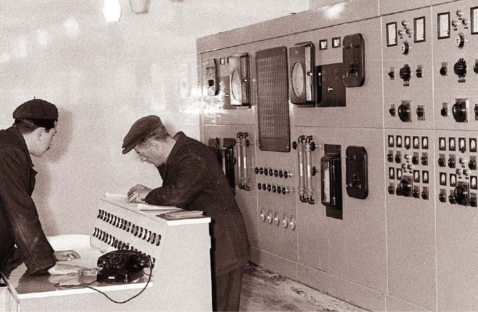
In the early part of the 20th century there were two sorts of control engineers. The first and largest group were from the mechanical and electrical industries, including the military, while the second were in process industries. The same principles were understood (or not) in quite different ways. For example, maintaining the voltage under varying current was equivalent to maintaining pressure under variable flow, but the technology was totally different. In 1911, Edmund A Sperry (1860–1930) produced an automatic gyroscopically stabilised steering system for the US navy, which incorporated full PID control with automatic gain adjustment (as understood in hindsight by modern engineers). He later adapted it for aircraft, and his son, Lawrence, produced the first autopilot. Sperry also invented processes for the manufacture of caustic soda, and for tin recycling, built an electric car which he drove in Paris in 1896, and demonstrated a radio-controlled “ariel torpedo” in 1918.

Many production processes operated in a sequence, and the same principles and technologies could be applied to batch chemical processes, with relays operating electrically powered pumps, valves, and agitators, according to time, temperature, level etc. These could be adapted to new electric signals such as pH, but customers in many process plants were used to pneumatic systems and had staff who could maintain them, so L&N sold pneumatic controllers for pH.

Between 1930 and 1940, automatic controls in US oil refineries doubled the capacity which could be achieved for the same dollar investment.
In 1951, a US company designed an oil refinery to be used in Asia. The government officials in charge asked for most of the automatic controls to be removed to provide employment for thousands of people to monitor gauges and operate switches and valves, saying they were willing to accept lower performance and quality for this reason. After careful study, the designers replied that it was impossible: plants now depended utterly on automatic control.

But perhaps not everywhere. In 1952, the journal Scientific American lamented “the unhappy situation of Great Britain. In spite of having…some of the best-informed technologists…her industrial leaders…have failed to understand the philosophy of automatic control.”

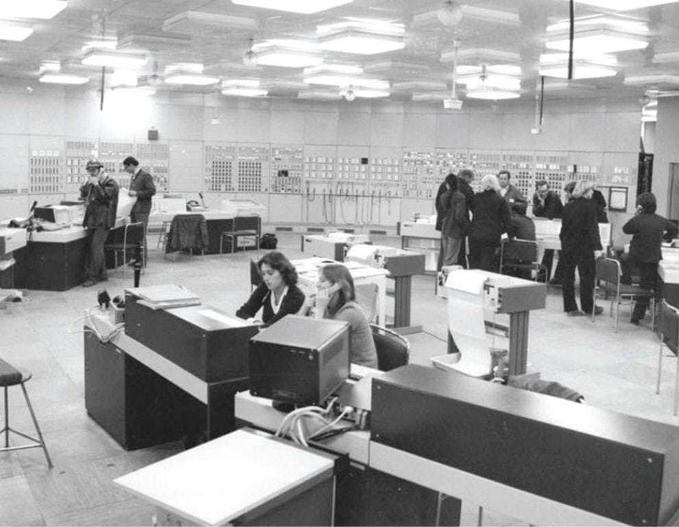
Computer control

In 1953, Simon Ramo (1913–2016) and Dean Wooldridge (1913–2006) left a company making real-time controls for missiles and set up Ramo-Wooldridge (later TRW). They built the Pioneer 1 spacecraft but also marketed the first computer for process use, the RW-300 which went fully online on 12 March 1959. It ran a catalytic polymerisation unit at Texas Co’s Port Arthur refinery with a state-of-the-art 8K memory and cost US$98,000 (about US$1m today) but improved the conversion of propylene to gasoline from 80% to 91%, paying for itself in less than three years.

In January 1960, another RW-300 ran an entire Monsanto ammonia plant. Two years later in Britain, ICI installed a Ferranti Argus 200 on a soda ash plant on Fleetwood, Lancashire. It had 209 inputs and operated 90 control valves and was identical to a computer used for the UK Bloodhound 2 guided missile. By 1965, the US had 400 such computers, the UK 54.

There had been computers on plants before, generally analog ones, to do the complex calculations for engineers to decide on process tweaks, and there was some competition for control. The Space Shuttle included an analog control computer, but progress and cost reduction meant digital won this particular race.

At this point, the process stream analyser was as key as the chart recorder had been. Feedback control on process parameters was not enough. Measuring the quality of the product and completing the mass balance was the ultimate feedback if it could be applied swiftly enough. The RW-300 did it every hour, adjusting 19 parameters (it may have made use of the principle of evolutionary operation (EVOP), published in 1957 by George EP Box (1919–2013), a statistician at ICI).

Two analysers were particularly important for the oil industry. The first mass spectrometer was invented in 1918 by Arthur J Dempster (1886–1950), greatly developed during World War Two, and was adapted for the oil industry in the early 1950s. The gas chromatograph was invented in 1954 by Archer JP Martin (1910–2002). The following year, Industrial & Chemical Engineering News outlined how useful it would be as a process analyser and by 1957 there were units on the market. Being able to monitor the composition of several components simultaneously was a huge advantage for the petroleum industry and provided a strong reason for adopting computer control, which boomed.

Meanwhile, in the 1960s motor industry there was a high degree of automation, controlled by a huge cabinet filled with relays clicking to operate machines via a forest of wires. To change to a new model essentially meant a complete rebuild, so in 1968 General Motors asked companies for ways to replace the cabinet with what they called a “smart machine controller”. Richard E Morley (1932–2017) won the contract with what was eventually called the programmable logic controller (PLC), essentially a small, rugged computer that only ran one program, in which a series of inputs would lead to outputs.

The PLC could be programmed by text instructions familiar to computer geeks. However, it could also be programmed by functional block diagrams, a development of the flowchart invented in 1921 by Frank Gilbreth (1868–1924) and Lilian Gilbreth (1878–1972), and therefore routine for production engineers. In addition, it could be programmed graphically in a way in which electricians could understand, using symbols for relay systems in what is called ladder logic (still in use today). While initially designed for production industries, the link between input and output could be extended to PID (proportional integral derivative) controllers ushering in their rise to prominence in the process industries.

The first process control computers were supervisory. That is, they adjusted setpoints on pneumatic or electric controllers. Thus, the plant would keep working if the computer was off, or being used for something else, as they were for many uses, including modelling, and preparing for shutdowns.

However, the PLC was direct control. Its instructions led directly to machine action. Modular units of many PLCs, each controlling some part, made fault-finding and fixing vastly easier than the previous system.

As digital computers got faster, cheaper, and more reliable, there was a move to eliminate PLC controllers and have all actions under direct digital control (DDC) of a single computer, with a major conference held on the subject in 1962. Within a few years, several manufacturers were offering minicomputers with this capability. It was generally taken up for large-scale heating, ventilation, and air conditioning (HVAC) systems, but there was some reluctance in the process industries with its extensive base of pneumatic and analog electrical systems, and fear of failure of the main computer.

In 1965, International Controls produced a supervisory control and data acquisition (later called SCADA) purpose-made computer for pipeline systems. The key to this was long-distance telemetry, which is still used for many small, separate PLC stations, and now being applied to larger plants.

In 1975, Yokogawa introduced both the name and the first distributed control system (DCS), followed by Honeywell and Bristol systems the same year. Yokogawa’s system, like the RW-300, adjusted independent controllers, plus a lot more. In the years that followed, cheaper microcomputers and microprocessors allowed redundancy, and a greater flow of information to and from “smart” instruments and controllers and all was well.

Or perhaps not. The issue was the means to transfer oodles of digital information, a problem that was also true for other data systems. Thankfully, Ethernet was invented in 1983 and standardised in 1985, becoming common for general business applications. Naturally, factories liked having the standard equipment and protocols for digital transmission in their offices and their plants. At about the same time, Rosemount developed the highway addressable remote transducer (HART) protocol, which could run on 4-20 mA wires at the same time as the analog signal, excellent for adding to existing chemical engineering plants. If two incompatible methods weren’t enough, in the 1990s there came what were called the “Fieldbus Wars” with different manufacturers pushing different digital transmission systems, and 20 industrial standards.

Though things are far from settled, the last 20 years have seen increased interoperability between equipment from different vendors and transmission systems, with benefits to users. Following last month’s feature on AI in TCE, you might wonder what it will do to process control. The answer is, it already happened in the 1980s, with self-tuning controllers using fuzzy logic and the first computer using expert systems to control 20,000 signals and alarms in a Texaco refinery in 1984. It, and others were built by Lisp Machines Inc (LMI), a spinoff from MIT’s AI laboratory.

In the 1991 film Terminator 2, the android (Arnold Schwarzenegger) explains that he can learn because he has a neural network. In the same decade, neural networks became popular for process control applications. In 2003, MS Office introduced an assistant in the form of an animated paper clip, an intelligent user interface (IUI). IUIs were increasingly used in computer control systems to assist the operator in, for example, detecting faults or prioritising alarms.

In fact, for the past two decades, most major process control systems have had some kind of AI components. Increasing computer power and software development will certainly add to this, but for some, the future is already here.

---

Read other articles in his history series: https://www.thechemicalengineer.com/tags/chemicalengineering-history