Practical Process Control Part 23: Inferentials in Action

The last three articles described the principles underlying the development and installation of inferential properties. Here, Myke King presents examples, selected to illustrate some key issues

ONE OF the problems in developing an inferential is deciding if any of the data should be rejected as outliers. While there are several statistical methods designed to help with this, there is always the risk that valid data are omitted. This could result in the inferential becoming unreliable when it is most needed – when the operating conditions shift away from typical values.

We include here, as an example, the development of an inferential on a LPG splitter. Figure 1 shows the requirement to infer the C₄ content (y) of the propane product. Among the potential independent variables are temperatures (x₁ and x₂) measured on trays 15 and 17.

Table 1 shows a selection of data collected from the process.

Regression gives two possible single-input inferentials, depending on which tray temperature we use:

Key to a successful inferential is ensuring it makes engineering sense. This is why development should fall into the remit of an experienced chemical engineer! The engineer would first ensure that variables are only included if they would be expected to affect the predicted property (we showed in TCE 1,005 how the inclusion of even a random measurement might appear to improve accuracy). Secondly, we check that their coefficients have the correct sign. In this case we would expect the C₄ content of the propane to increase with tray temperature and so the positive coefficients make sense. We also must justify, from an engineering standpoint, choosing the inferential with the higher R̅². In this case we would expect a closer correlation with the temperature higher up the column.

The next consideration is whether additional independent variables should be included. In this case, should we include both temperatures? Our first reaction might be not to do so. They are on almost adjacent trays and will therefore be highly correlated. If one temperature can be represented as an exact linear function of the other, then its inclusion will not improve accuracy. Figure 2 appears to confirm that this is the case – apart from two points which we might consider as outliers.

However, if we include them in the regression, we obtain:

Examination of the coefficients might, at first, give us cause for concern – since that of x1 is now negative. But, before rejecting the correlation, we should attempt to understand the cause. In this case, we can rewrite the equation as:

Figure 3 shows two temperature profiles – one for less pure and the other for almost pure products. It shows how (x₁ – _x2) is a measure of component separation. The greater the temperature difference, the more closely the boiling points of the products approach those of the pure components. So, the C₄ content of the propane reduces – explaining the negative coefficient.

It is important that the temperatures are close together. Installed on trays wide apart they could still be a valuable input to the inferential but will cause problematic dynamics. For example, Figure 4 shows the result of a disturbance occurring near the base of the column (say a change in reboiler duty) where the temperature of the lower tray changes before the other.

Incidentally, inclusion of temperature difference is usually beneficial on most columns. But rarely are multiple temperatures installed, and they are too costly to retrofit. A lesson learnt in involving experienced control engineers in process design – identifying the need during process design would add little to cost and might capture substantial benefits.

Transformations

While we generally use linear regression analysis to develop inferentials, we can selectively first apply non-linear transformations to both the dependent and independent variables. For example, rather than trying to predict the concentration of an impurity (C) in a distillation production we instead predict log(C). For high-purity columns, this helps linearise very non-linear behaviour. It also has the advantage that the predicted concentration cannot be negative. If we do predict log(C) we apply the inverse transformation to the result before displaying it to the operator.

We can also apply transformations to the independent variables. One example we covered (see TCE 996) was using the logarithm of absolute pressure in inferentials that rely on a pressure compensated temperature (PCT). PCT is also an example of a compound variable. Although appearing in the inferential as a single input, it is derived from two raw measurements – column pressure and tray temperature. Other common compound variables are flow-to-feed ratios, where the flow might be a product or a utility stream. The use of the ratio helps make the inferential immune to changes in feed flow.

Reactor conversion will generally depend on residence time. We would then see the benefit of using the reciprocal of the feed flow. Indeed, liquid hourly space velocity (LHSV), defined as the hourly volumetric flow per unit volume of catalyst, will often appear in an inferential as LHSV^-1.

Reactor temperature

A process, common throughout the oil industry is the hydrotreater – often used to produce diesel. Raw feedstock is reacted with hydrogen at a high temperature over a catalyst. Feedstock derived by fractionating crude oil compromises saturated (paraffinic) hydrocarbons. Components produced by cracking larger paraffinic molecules are unsaturated (olefinic). Feedstock for biodiesel production is also largely olefinic. The purpose of hydrotreating is to first remove sulfur compounds (mainly mercaptans). Secondly, olefinic components are saturated to meet the required bromine number (a measure of unsaturated hydrocarbon content). Reactor temperature is the key variable in determining product composition. Usually this is controlled by manipulating the fuel flow to the upstream fired heater. When processing paraffins there will be a small temperature drop across the reactor but, due to the exothermic nature of hydrogenation, there will be a substantial increase when processing olefins. The mixture of feed components can change. When it does so, the reactor temperature profile will change and so affect product composition. The residence time through the process is typically around 90 minutes. An inferential property measurement, based on reactor conditions, would give an indication of change much sooner than an analyser on the reactor product. The key (and often only) input to the inferential is the equivalent isothermal temperature (EIT). As its name suggests, this is the temperature. If the same throughout the reactor, that would give the same conversion as the current temperature profile. It is defined as the weighted average of RIT and ROT – the reactor inlet and outlet temperatures:

We determine x by developing the inferential for the product quality:

While we could implement the inferential as defined, a more elegant solution is to install an EIT controller, as shown in Figure 5 – particularly if it is the only input to the inferential. This will maintain the EIT constant as the composition of the feed changes.

The equivalent for multi-bed reactors is the weighted average bed temperature (WABT), where each bed inlet temperature (T) is weighted depending on the quantity (w) of catalyst in each bed:

Again, rather than use the weight of catalyst, the coefficients would be determined by regressing Q against T₁, T₂, T₃ etc. The first reactor inlet temperature (T₁) controller would be replaced with a WABT (weighted average bed temperature) controller.

In many reactors the catalyst deactivates over time. In the case of the hydrotreater, the EIT must be gradually increased to meet the product quality target. When reaching its upper limit, the catalyst is either replaced or regenerated. During the run length the correlation between product quality and EIT will change and so the inferential will need regular updates to its bias term. Rather than accept this, we should strive to build into the inferential some measure of catalyst deactivation. One approach would be to maintain a record of the total feed processed since the catalyst was fresh. Regressing with this as one of the inputs would likely remove the need for bias updating.

Consistency with MPC

Inferential properties are frequently control variables (CVs) of a multivariable predictive controller (MPC). Included in the dynamic models used by the controller are the steady state process gains (K_ij) between the CVs and the manipulated variables (MVs). Table 2 shows the gain matrix for such a controller.

It predicts the steady state from:

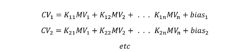
If CV₁ is an inferred property then, if linear, it will have the form:

It is highly likely that some of the x variables will also be MVs. If all are MVs, then it is important that the two predictions are consistent, ie a₁ must be the same as K₁₁ etc.

SP or PV

If an input to the inferential calculation is a variable which is controlled with a proportional-integral-derivative (PID) controller, we have the option of using either the PID setpoint (SP) or its process variable (PV). The use of SP has advantages. Firstly, it will be noise-free. But more important is that the inferential will not change if there is a process disturbance that will soon be corrected by the PID controller. Were it do so, it would make unnecessary corrections that would ultimately have to be reversed. Figure 6 shows a typical arrangement.

A quality controller, say on a distillation column, is cascaded to a tray temperature controller (TC) which, in turn, is cascaded to a flow controller (FC), perhaps on reboiler steam. The problem is that, if the operator changes the SP of the quality controller, it will immediately change the SP of the TC, which will immediately change the SP of the FC. Since these SPs are inputs to the inferential calculation, the process variable (PV) of the quality controller will change immediately. As far as the quality controller is concerned, the process has no deadtime (θ) and no lag (τ). Controller tuning calculations are based on the θ/τ ratio, which would be indeterminate. It may not be possible to tune the controller, even by trial-and-error, to give satisfactory control. One solution would be to filter the quality controller’s PV to introduce a lag (τ > 0). Of course, this might be counter-productive – undermining the advantage of rapidly responding inferential. Or we may have to abandon the use of SPs as inputs and instead use PVs.

The topics featured in this series are covered in greater detail in Myke King's book, Process Control – A Practical Approach, published by Wiley in 2016.

---

This is the twenty third in a series that provides practical process control advice on how to bolster your processes. To read more, visit the series hub at https://www.thechemicalengineer.com/tags/practical-process-control/

---

Disclaimer: This article is provided for guidance alone. Expert engineering advice should be sought before application.