Practical Process Control Part 17: Fired Heaters - Part 1

In the first of a two-parter on fired heaters, Myke King shows how to implement duty controls

PERHAPS the most common technique for measuring gas flow is the orifice type flow meter. The orifice acts as a restriction; the pressure drop across which is indicative of flow rate. The instrument engineer, when designing the meter, will have used design conditions for molecular weight (MW_design), pressure (P_design), and temperature (T_design). These values will have been used to determine the meter constant – the flow in engineering units when the meter records 100% of range. This factor is then used within the DCS to display the current flow (F_measured).

Of consideration, if the gas is a fuel, is its heating value. There are two measures of this. Here we will use net heating value (NHV) – on the basis that any water produced as a combustion product stays as vapour. Should the water be condensed, then the larger gross heating value (GHV) would be applicable.

Flow meter correction

Of course, actual operating conditions can vary from design conditions. If we have measurement of the current conditions, we can use them to correct the flow measurement.

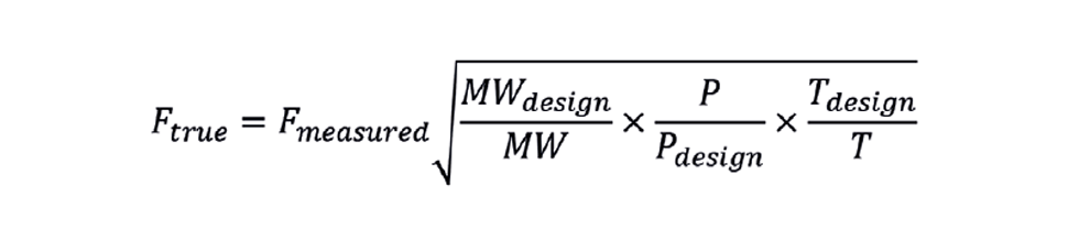
Both pressure and temperature must be in absolute units, but we can usually omit the temperature correction. Imagine that the design temperature is 25°C and the current temperature is 30°C, then the correction factor would be the square root of (25+273)/(30+273), or 0.992. This correction of 0.8% is less than the flow meter reproducibility. Further, including temperature increases the likelihood of losing the flow measurement through instrument failure.

This formula is applicable to any flow meter that relies on generating a pressure drop as an indication of flow. In addition to orifice types, this includes pitot tubes, annubars, and venturi. The equation is written assuming that the flow is reported in volumetric units at standard conditions (eg sm³/h at 1.01325 bara and 15°C) rather than actual conditions. However, it could be a mistake to apply it to a fuel gas meter. On many sites, fuel is a variable mixture of components – perhaps byproducts of a number of process units, possibly supported by imported natural gas. Let us imagine that the composition of the gas has changed so that the molecular weight increases. F_true will therefore fall. If there is a flow controller, it will take corrective action and open the control valve. However, increasing molecular weight usually indicates that the NHV is increasing. Instead of the valve opening, we should be closing it to maintain a constant duty. Adding this correction term to an existing flow controller will worsen control of the heater.

In the equation above, we can replace MW with specific gravity (SG), where:

Analysers measuring SG are available, with a total installed cost similar to that of a flow meter. Often described as a densitometers, it is important the model chosen measures density at standard conditions, not at stream conditions.

Compensation for NHV

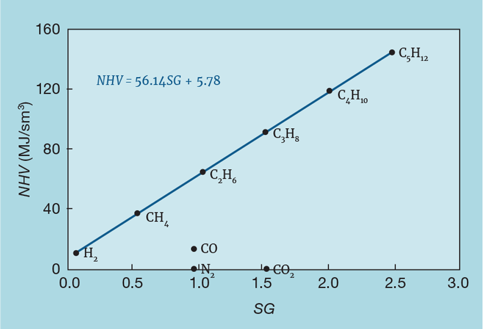
Figure 1 shows the relationship between NHV (in MJ/sm3) and SG for pure components. In principal, measuring SG, required for the flowmeter correction, also allows us to infer NHV. As shown, we can calculate the coefficients 56.14 (a) and 5.78 (b) from the physical properties of the components. However, site fuel gas systems can contain small quantities of other gases that don’t match the prediction. These might have zero heating value, like CO2 and N2, or not be hydrocarbons, like CO. We therefore have to develop a correlation for the site in question. Most sites will routinely sample their fuel gas system, analysing the gas in the laboratory to give a full component breakdown. From this we can calculate NHV and SG.

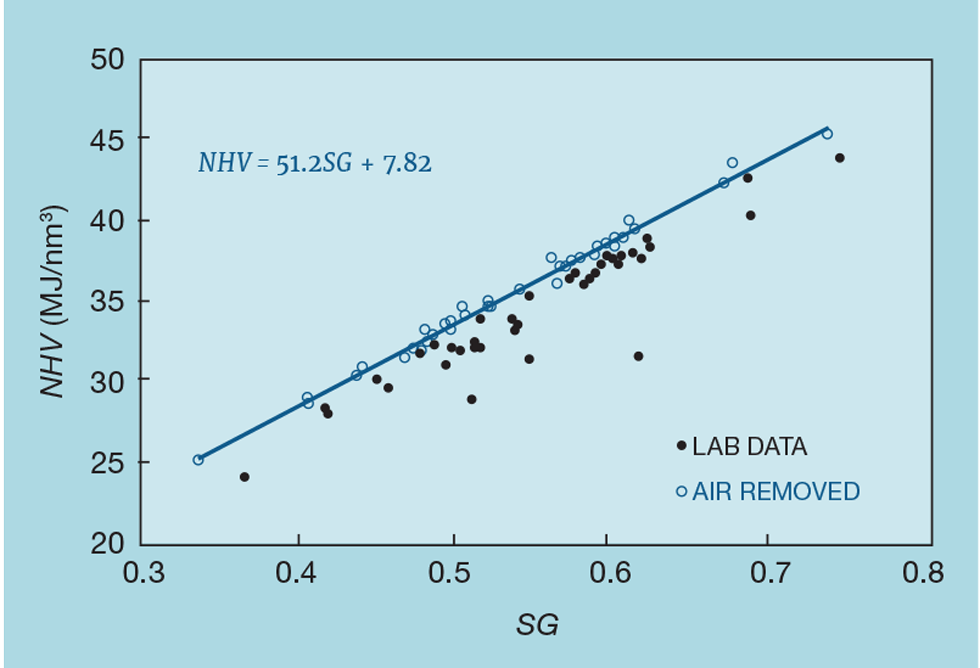
Figure 2 shows such data. The original data (the solid points) show a poor correlation, but examination of the analyses shows that oxygen is regularly one of the components. Unlikely to be present in the site’s fuel system, it has been introduced by the sampling procedure. We can readily remove it from the calculation of NHV and SG but, since it was introduced as air, we also remove the associated nitrogen – calculated as 3.73 times the oxygen content. Fuel gas can genuinely contain nitrogen, so some is likely to remain after removal of the air. Figure 2 shows the impact this technique has on the correlation – resulting in a reliable inference of NHV.

By multiplying the corrected flow by the inferred NHV, we obtain the process variable (PV) for the fired duty:

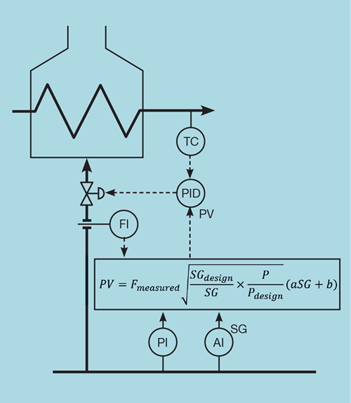
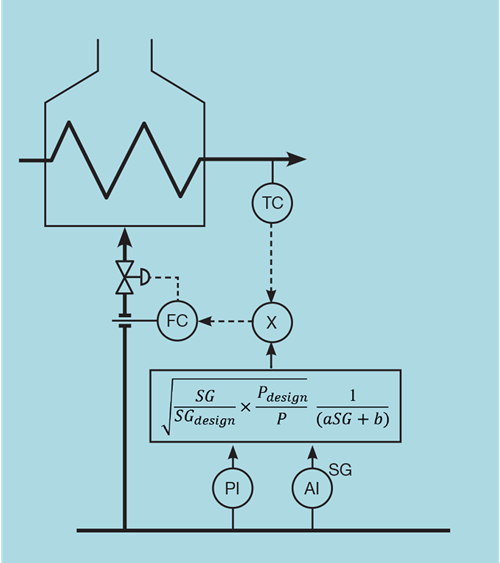
Examination of this equation shows that, on increasing SG, PV will increase. If now used as the measurement of a controller, this will close the control valve as required.

Figure 3 shows how the scheme would replace the flow controller. 

Alternatively, if the preference is to retain the flow controller, we can invert the correction. Multiplying the output of the temperature controller (the duty demand) by this factor then converts it to units of gas flow, as shown by Figure 4.

Analyser installation

It is common for several heaters to take fuel from a common gas header. We do not therefore need an analyser on each heater. However, the impact of an analyser failure could then be quite severe – potentially affecting every heater and boiler on the site. Further, some of these heaters could be on plants that produce some of the fuel gas and so propagate the disturbance to the site fuel gas composition. Under such circumstances it is advisable to install multiple analysers and cross-check their measurements.

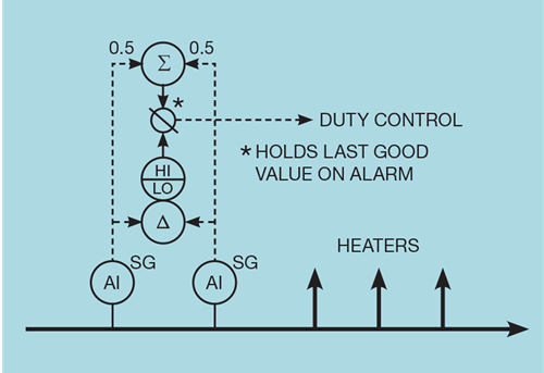
Figure 5 illustrates one possible approach, employing two analysers. Normally the average of their measurements is used but a large difference between them is treated as a failure. The value then used for control is frozen at the last good value. This gracefully degrades the duty controller – retaining all its other features. We would need to decide on what action should be taken when the analysers are again working. If the SG has changed during their omission, then the feedback controller will have adjusted the duty controller setpoint. Recommissioning analyser correction will be treated as a change in SG and will unnecessarily bump the process.

Some mechanism needs to be in place to prevent this. One possibility is that the duty controller must first be switched to manual mode. Returning it to auto, with the SG correction in place, will reinitialise the controller.

Mass flow

Of course, we can choose to calibrate the meter to report mass flow, in which case the correction becomes:

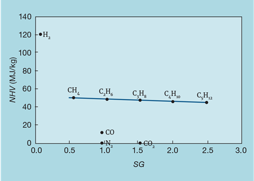
Figure 6 shows the relationship between NHV (now in mass units) and SG. Provided hydrogen is not present in significant quantity then the NHV changes little with composition. So, by choosing a flow meter that directly measures mass flow (such as the Coriolis type), we do not need a SG analyser (while most Coriolis meters also provide a measure of density, this is determined at stream conditions and so, unless pressure and temperature are measured, cannot be used to infer MW or NHV).

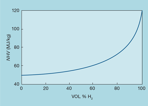
Fuel gas analyses are commonly reported on a volume basis. When deciding whether the presence of hydrogen significantly affects the applicability of mass flow metering, we need to convert the analysis to a mass basis. Figure 7 shows the impact of hydrogen content on NHV, when mixed with the lightest hydrocarbon, methane. For example, if the hydrogen concentration were to vary in volume between 10 and 20%, it would cause a ±1% change in NHV. Mixed with heavier fuels, the impact of hydrogen would be even less.

Wobbe index

In the unlikely event that NHV cannot be inferred with sufficient accuracy then there are on-stream calorimeters available. These are considerably more expensive than SG analysers – both to purchase and to install. They will also be slower – potentially correcting the fuel flow after the feedback controller has already taken corrective action, and so cause a second disturbance. They are often described as Wobbe index (WI) analysers, where:

The duty calculation then becomes:

Sample timing can also be an issue with SG analysers. On sites with very long fuel gas headers, they can be installed potentially too far upstream. Indicating a change in gas properties long before the fuel reaches the heater will cause flow correction too soon. The feedback controller will respond to the disturbance this causes but will then have to undo this correction when the change in fuel gas composition reaches the burner. The resulting process upset can be worse than that where no on-stream analysis is available. While one might consider using the control system’s deadtime algorithm to add an appropriate delay to the analyser measurement, this is rarely practical. The required delay will vary with fuel gas flow rate. Further, on complicated headers, the route taken by the gas can vary. In practice it is better to install individual analysers for each heater, placing them at a suitable upstream distance.

---

The topics featured in this series are covered in greater detail in Myke King's book, Process Control – A Practical Approach, published by Wiley in 2016.

---

This is the seventeenth in a series that provides practical process control advice on how to bolster your processes. To read more, visit the series hub at https://www.thechemicalengineer.com/tags/practical-process-control/

---

Disclaimer: This article is provided for guidance alone. Expert engineering advice should be sought before application.