Practical Process Control Part 20: Regression Analysis

Inferential properties, or soft sensors, are key to modern process control. Myke King explains regression analysis as a precursor to their design

TO PLAGIARISE from a much longer quotation by Lord Kelvin, if you cannot measure it, you cannot improve it. But direct measurement, by an on-stream analyser, can be expensive, unreliable, and slow.

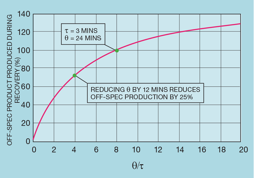
While analyser technology is improving and, importantly, more attention is paid to the sample system design, inferential properties will always have a place – if only because they respond far quicker than most analysers. Indeed, to ensure earlier correction of off-spec production, an inferential will usually be installed in addition to the analyser. The analyser’s role then becomes one of trimming the inferential calculation to maintain its accuracy. Figure 1 illustrates the benefit of this approach. Analysers tend to exhibit long delay, or deadtime (θ). In our example, the deadtime-to-lag ratio (θ/t) is 8. This is typical of a chromatograph on a distillation column overhead product. As a base case we define 100% as the amount of off-spec production following a process disturbance, assuming an optimally tuned product quality controller. If the installation of an inferential halves the deadtime, then the controller can be more tightly tuned and off-spec production reduced by 25%.

The choice

There are two types of inferential. The first-principle type employs semi-rigorous modelling techniques, akin to those used in process simulation. The models tend to be complex, proprietary, and more demanding of technical support. While, for some applications, they can outperform the regression-based type, they form a small minority of installed inferentials. In the next four articles we focus on regression.

The problem

Regression analysis takes historically collected process data to develop a correlation between the property we wish to control (the dependent variable) and process measurements of flow, temperature, and pressure (the independent variables). While most inferentials predict the property of a product, most commonly on distillation columns, there are other applications. Common are those that measure catalyst activity and reactor conversion. One could also consider the more advanced compressor anti-surge techniques, that we will cover in a future article, as inferentials.

There are a range of platforms available – including Aspen IQ, Honeywell’s Profit Sensor Pro, and Shell’s RQE. These are installed in the process computer interfaced to the distributed control system (DCS). They are used to both develop and host the inferential. But much can be accomplished using the standard features of Excel and then installing the inferential within the DCS. The ease with which multidimensional regression can now be applied can lead inexperienced engineers into developing inferentials that are insufficiently accurate. Indeed, audits completed by the author's consultancy would suggest that well over half of those installed would achieve greater profit improvement by being decommissioned! So, the purpose of these articles is to take the reader through the development methodology, dispelling any myths about how accuracy is tested and maintained – and to show how performance should be properly monitored and improved.

The basics

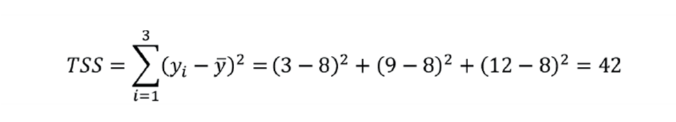
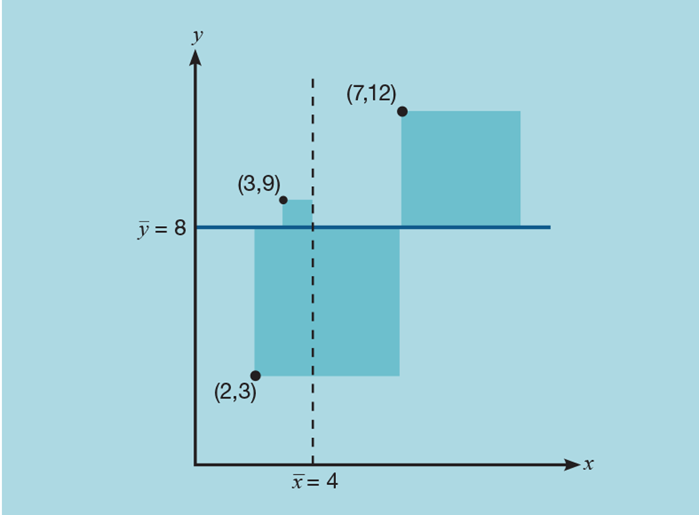
Let us take a very simple example, as shown in Figure 2. We have three points plotted as xy coordinates – (2,3), (3,9), and (7,12). To perform the regression, we first determine the mean of both x and y; so (x̅,y̅) is (4,8). From this we can calculate the total sum of squares (TSS), shown as the shaded area:

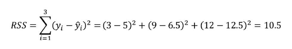
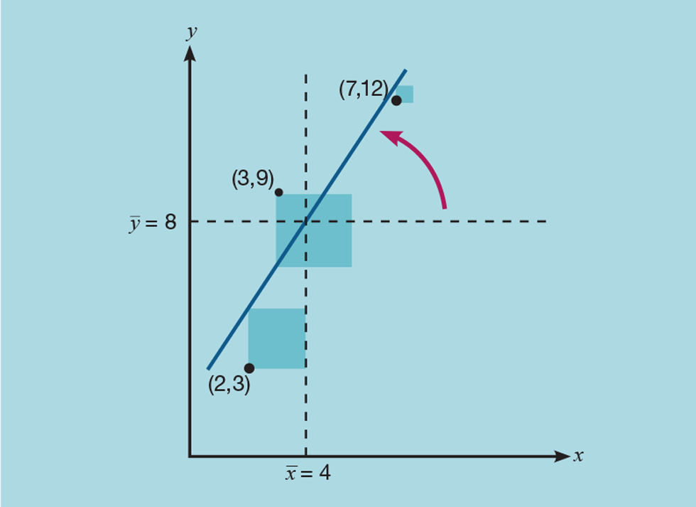
As Figure 3 shows, we then rotate the line passing through (x̅,y̅) to minimise this sum. We could use Excel to show that the equation of the line of best fit is:

The shaded area is now the residual sum of squares (RSS):

It is this value that regression analysis has minimised. To assess how well the equation fits the data we determine the explained sum of squares (ESS):

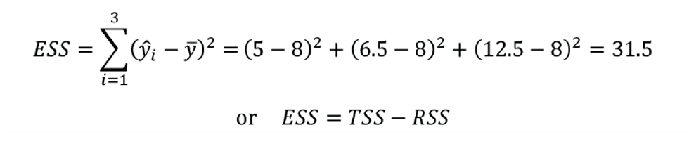
The fraction of the variance explained is the coefficient of determination:

This is a measure of how well the predicted ŷ matches the actual value of y. But is one of several definitions of R². That more commonly used was defined by English biostatistician and mathematician Karl Pearson as:

The value determined by this method is also 0.75. This is because we are applying it to the data used to develop the inferential. If applied to monitor the reliability of a previously developed inferential, the two definitions will give slightly different results. So, which should we use? The first definition might appear more intuitive, but it suffers a major drawback. If we were to shuffle the order of the actual values of y, leaving that of the predicted values unchanged, then R² does not change. It’s basically telling us that, provided today’s inferential agrees with the actual property that might have been measured a few days ago (or in the future), then it’s good to use in a control scheme! The second definition does properly reflect the time series nature of process data.

Why do we base the penalty function on the dependent variable (y)? By doing so, we are assuming that its measurement is perfect, and we want to get our prediction as close as possible. But it may be that we have greater confidence in the measurement of the independent variable (x) and want to stay as close as possible to its value. In which case we should minimise:

This would give the line of best fit as:

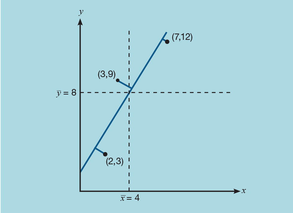
Or maybe we have equal confidence in the measurements of both x and y – in which case we might minimise the sum of the squares of the perpendicular distances, as shown in Figure 4. For example:

So, does R² tell us which of the three equations is the best fit? Well, no; perhaps surprisingly it has the same value for all three. In fact, we can choose any linear function of x and we will get the same result. R² tells us only how closely x and y are correlated; it tells us nothing about the reliability of the inferential.

This issue is only apparent for inferentials based on a single independent variable. But this input can be a compound variable derived from two or more measurements. For example, the composition of a distillation product might be inferred from a pressure-compensated tray temperature (see TCE 996) or maybe reflux ratio. There are many such suspect inferentials in place.

We can use weighting factors (w) to select the penalty function. For example, if we have two independent variables, our inferential would take the form:

To determine the a coefficients we would minimise:

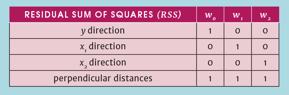
Table 1 shows the impact of the weighting factors. Values of w are not restricted to 0 or 1. For example, if we felt that x² was more reliably measured than x₁ we might assign a value to w₂ that is higher than that for w₁. Another limitation of R² is that we cannot use it to choose the best values for the weighting coefficients. The way it is defined means that it will always result in a value of 1 for w₀ and 0 for all the others.

Avoiding pitfalls

Including additional measurements in the inferential leads us to another problem with the use of R². Imagine we develop a correlation that includes m independent variables, and we use n records of historical data. If n is equal to m + 1, then it would be possible to choose values for the a coefficients such that we obtain a perfect fit to the data. The most trivial example would be to plot y against x using only two sets of data. The correlation would pass exactly through the two points. While extreme, it illustrates that, if too few records are regressed, the estimate of R² will give an optimistic assessment of the correlation. The solution is to determine the adjusted R²:

This equation can be used to assess whether we have included enough data in the regression. If significantly increasing n has little impact on R̅², then we can deduce that n is sufficiently large.

Now, to illustrate another problem, imagine we have developed an inferential using only x₁ and we wish to explore whether the addition of x₂ would be beneficial. In fact, no matter what that measurement might be (even if it is a random number!) the value of R² will increase. This has caught out many an inexperienced engineer who has “thrown” data at regression analysis and naively developed an inferential that, when installed, generates a largely random result. Again, using adjusted R² helps resolve this. If we find that increasing m reduces R̅² then the additional input has no place being included in the inferential.

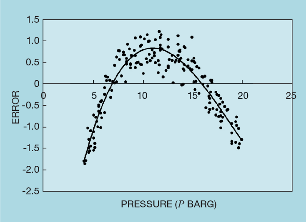
We can also check whether an input has been overlooked – by plotting the error in the inferential against each unused input. If this shows any correlation, then the input should be included. The same technique can be applied to those inputs already included. Figure 5 shows an example of column pressure that is already included in a distillation inferential. While accurate at two pressures, its shape indicates that some non-linear function of pressure should be considered. Commonly, as we saw in TCE 996, using its logarithm will improve accuracy.

Finally, we have to address the scatter of the data used. Process operators are generally good at keeping a product on grade by making manual adjustments, based on the result of a regular laboratory test. This means the variation in the process data may be insufficient to develop a reliable correlation. Let us imagine we wish to explore the reliability of an inferential that predicts the C₃ content (Q) of the butane product from a liquefied petroleum gas (LPG) splitter, based on a tray temperature (T) in the lower section of the column:

From the data used to develop the inferential we first calculate:

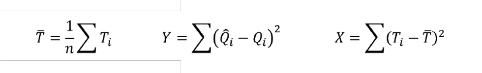
For the feasible range of values of T we plot Q̂̂ and Q̂ ± E:

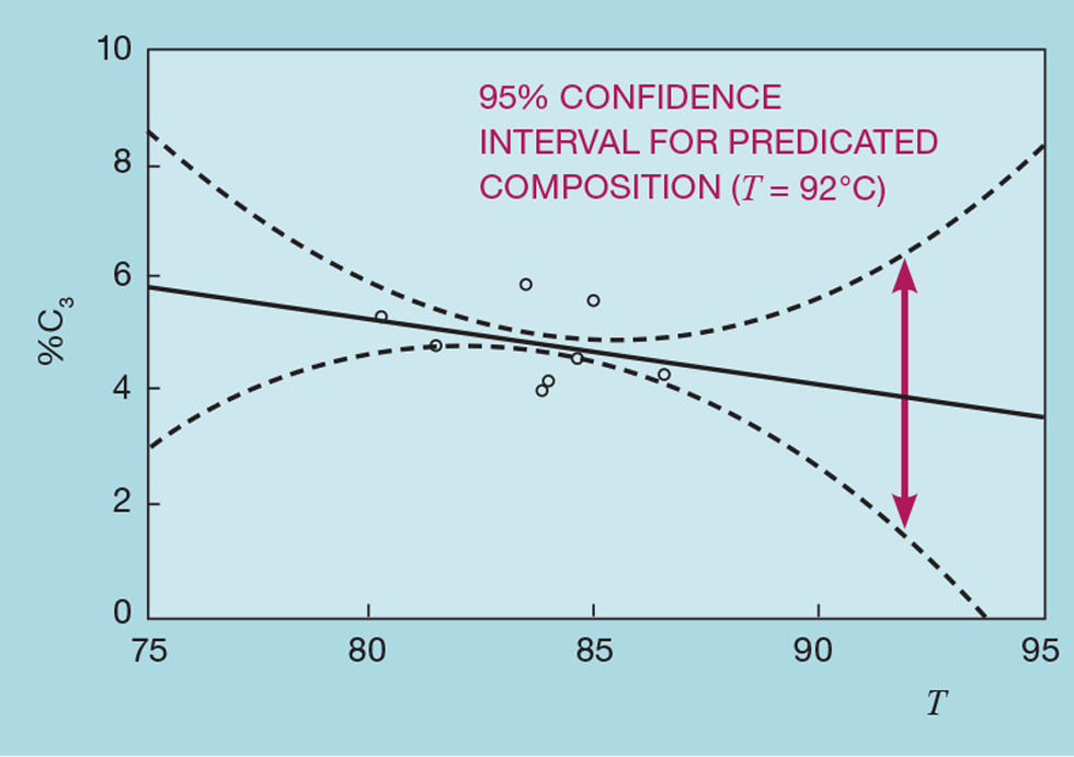
Figure 6 shows the result – with inclusion of the original process data (shown as individual points). The solid line is the predicted composition, while the dashed lines represent the envelope within which we are 95% confident the solid line lies. So, if the tray temperature were 92°C, we would have very little confidence in the predicted composition of 4% C₃. There simply is not enough variation in the data used to build the inferential. We would need to conduct test runs to collect data well away from the target operation.

From the equations above, it would appear the check on scatter can only be applied if the inferential includes a single independent. However, we can condition each independent to take account of the variation in the others. For example, if our inferential has three inputs and we want to assess the scatter of x₂ then we first condition it as:

The topics featured in this series are covered in greater detail in Myke King's book, Process Control – A Practical Approach, published by Wiley in 2016.

---

This is the twentieth in a series that provides practical process control advice on how to bolster your processes. To read more, visit the series hub at https://www.thechemicalengineer.com/tags/practical-process-control/

---

Disclaimer: This article is provided for guidance alone. Expert engineering advice should be sought before application.