Engineering Net Zero Part 9B: Modelling of our Energy System

David Simmonds offers a tool to simplify the presentation of the long-duration balancing measures needed for UK's future power system

IN PART A of this mini-series, I visualised the challenge for the last 20% of demand, by looking at system balancing measures to manage shortfalls and oversupplies from renewables. Here, I draw upon the experience gained balancing the NW European gas grid back in the 1990s when we used load duration curves. However, that example only considered dispatchable power, so we must address the added complexity of renewables intermittency.

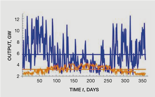
As we know, intermittency presents itself as a sawtooth profile over the year, exemplified here for wind in blue and solar in red, courtesy of David Dunstan at Queen Mary University. Looking at this it is difficult to see how balancing may work, so we need something better.    

Stochastic modelling and load duration curves

Modelling of our future energy system must consider the randomness of weather, with its impact on both demand and renewables supply, and a number of other parameters such as plant and grid reliabilities and availabilities. Deterministic approaches used for most decision-making does not work when we have these input uncertainties, and planners use stochastic models to manage them, such that a given set of input conditions will lead to a variety of outputs. The inherent randomness of the input data is defined through a set of probabilities to allow a Monte Carlo simulation of the design case. In short it needs good models and a lot of computing power, and I imagine it is an area where AI will assist in the future.

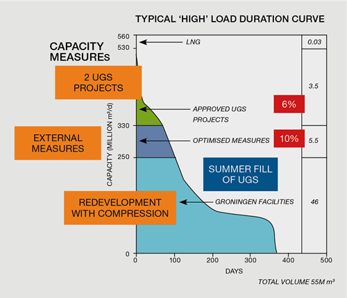
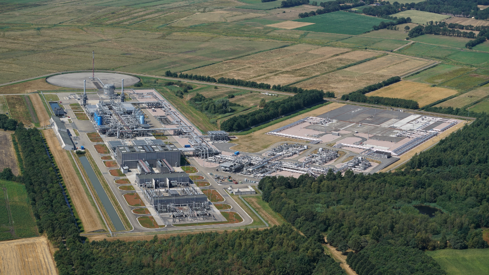
Working for Shell in the early 1990s, I supported Gasunie, the Dutch state gas entity, to scope and redevelop the Groningen field and build underground gas storage (UGS). These measures would ensure the field continued to meet demand criteria set by the state. We used stochastic analysis of weather-dependent demand and modelled system capacity. The analysis enabled us to produce a “high”, harsh winter, load duration curve (LDC) which orders daily demand by magnitude, rather than chronologically, for the 365 days of the design year. Simply put, we ran the system model say 1,000 times and used the output from the tenth-highest demand solution to determine the one-in-100-years design case. As can be seen, the beauty of the magnitude stacking of the results is that we can visualise the volumes involved, and size each capacity measure with its hierarchy in the LDC (note, we did not have to worry about in-day balancing as this was met by gas grid buffering). 

Can we develop such a stochastic LDC to better present the long-duration measures needed within our future power system?

Application of load duration curves to our power system

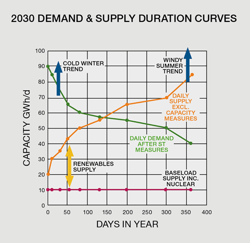
Unlike Groningen, our future renewable-based energy system requires stochastic analysis of both demand and supplies. Planners can produce an LDC (stochastic daily demand after short-duration, in-day, balancing measures) and a supply duration curve (SDC) showing stochastic daily supply of non-dispatchable power, nuclear and renewables, contracted under contracts for difference agreements. Like Groningen, demand data is day averaged.

Typically, the LDC and SDC would look as shown here, where the x-axis depicts each day’s energy sorted by magnitude through the year, with the y-axis as the daily power quantum, typically expressed in GWh/d. The sorted green demand curve (LDC) is comparable to the Groningen example, while the tan-coloured line represents a supply curve (SDC) of non-dispatchable power, stacked sequentially in magnitude in the opposite direction. Day 1 on the demand curve represents peak demand while Day 365 shows peak supplies. Cold winters and/or windy summers can markedly change the shape of the two curves.  

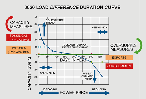
I hope it is obvious that the stacked supply and demand data do not coincide, so we must determine a better way to represent baseload, intermittent and back-up capacity measures on any given day. My lightbulb moment was to consider a load difference duration curve (LDDC), one which uses the demand and supply data for each day, calculating the difference for every day of the year. Sequentially stacking the results, by magnitude, similar to the Groningen LDC, creates a sideways, S-shaped curve, swinging around zero, the point at which both demand and non-dispatchable supplies are balanced.

As one can see, the LDDC for a given year displays shortfalls and excesses, with long-duration capacity measures, on the left (red arrow, typically days 1-90), and oversupply measures, on the right (green arrow, typically days 271-365), required to bring the system into balance each and every day. Days 91-270 require little balancing mainly achieved through short term measures including hydro.

The real benefit of this presentation is that it quantifies those measures and visualises the “skin” of the onion (the final 15-20% of demand) as described in Part 9A. As can be seen, in 2030, this is managed through use of the interconnectors with fossil gas generation as the final capacity measure and curtailments as the final oversupply measure. The chart also demonstrates the impact of demand-driven variable pricing, increasing during shortages and dropping with oversupply.

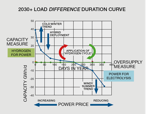
We also saw in Part 9A, the longer-term solution for managing peak demand is hydrogen, produced through the hydrogen cycle, and this too can be represented on the LDDC with surplus power used to produce hydrogen through electrolysis, and hydrogen-to-power used as the capacity measure, a cyclical process.

Given the current investment in interconnectors and the added diversity they offer, it clearly makes sense to keep import and export measures within the plan. Nonetheless, further investment in interconnectors must be compared to the circular benefits of the hydrogen cycle, something which I will consider in more detail in Part 9C.

As the Groningen LDC helped us scope measures, gas storage, and priorities for deployment, the LLDC can assist sizing of electrolyser, hydrogen peakers, hydrogen storage, and interconnector capacities. Further as will be shown in Part 9C it can also be used to show the benefits of hybrid technologies operating as a long duration (DSR) measure to reduce peak power demand.

The LDDC can be used to determine parameters for both average or typical weather years and more critically for cold winter or windy summer scenarios. Reserve storage volumes should also consider multi-year impacts, something the Royal Society addressed in their modelling, presented in Figure 2, page 11, of their full report.

Future commercial model

Today’s high cost of electricity makes UK industry unattractive for investment and directly impacts consumers’ cost-of-living. Renewable energy is cheaper than fossil energy, so we are on the right track, but keeping existing gas assets on standby and building new long-duration measures as foreseen above, add to their cost. Indeed, in chapter 9 of their report, the Royal Society concludes that the current commercial model for energy must change, and I can only but agree.

Renewables are being developed under a contracts for difference mechanism which provides pricing certainty for the generator (they carry wind and project risk, not offtake risk), but, as we have seen, leaves government exposed to curtailment fees when demand is low, or the grid is unable to cope with high generation on windy days. The new measures to reinforce the onion (to meet the 15-20% challenge) will be paid by government through capacity charges, but these will be passed through to bills, either as a fixed fee or, more likely, through variable or demand pricing. Battery projects such as the recently completed Blackhillock  project add significant cost to the consumer. A few such projects may well be needed to manage short-duration demand variations, but they are not the answer for long-duration balancing.

Variable pricing is already the standard for wholesale and industrial markets, and I have indicated trends on the LDDC. Selling surplus power to Europe cheaply over the summer will not compensate for expensive winter purchases. On the other hand, variable pricing will drive the economics of the inefficient hydrogen cycle, which, once established and being cyclical, will offer more resilient flexibility than interconnectors.

Developing a robust commercial business model which works for renewables investors, wholesalers, retailers, grid operators, industry, and consumers, while building a resilient system to cope with design winter demand and still meet net-zero targets, is the  challenge, and it can’t be delivered until we fully understand how our future energy system will work. We have already seen with storage of natural gas that maintaining contingencies for cold winters comes under economic scrutiny, especially when it is only needed irregularly. The same will be true for some of the new capacity measures in our power system, so in another recent article, I presented some thoughts on how Great British Energy could support balancing and capacity measures to reduce commercial risk and simplify investment structures. We cannot expect the private sector to carry usage risk of measures designed to cover harsh winters or other events such as the Ukraine war, which could in a particular year cost the UK £100m (US$127m) and/or fatalities from failing to “keep the lights on”.

Delivery of our future system

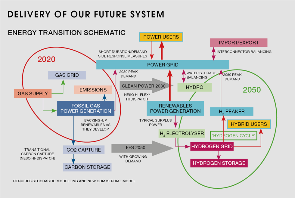
I started the ENZ series by looking at planning and collaboration, so I hope this analysis again brings this into the headlights. Chemical and electrical systems  engineers must work closely with our commercial and marketing colleagues to model, explain, and deliver a resilient, clean, safe, and commercially viable energy system. This chart provides another representation of the scope, including those essential load balancing and capacity measures.

Following presentation of the Power System Onion, I hope that the LDDC is a useful tool to help up quantify the measures needed to balance our future power system using the results from complex stochastic modelling. Planners can use this to share the challenges of designing a resilient energy system built around intermittent renewables, with, for example, the National Energy System Operator (NESO) using it to demonstrate the differences between and the workings of their 2030 options and 2050 scenarios.

In Part 9C, I will comprehensively examine these scenarios and compare them to a more flexible strategic alternative that can reduce costs and energy prices, enhance resilience, minimise local impact, and further decrease our dependence on imports.