Avoiding Modelling 'Magic Pressure Rises'

Introduction

The availability of easy-to-use process simulation software has made obtaining physical properties and compositions for a wide variety of systems, into a relatively simple and quick procedure.  However, the ease and speed of use all-too-often results in a lack of time spent understanding the results given out by the software, and questioning the validity of the data. It looks sensible, so why would the simulation be wrong?  A user can typically ask the software to provide a result regardless of whether it represents what a real system would do, for example specifying a heat exchanger duty that would cause a temperature cross.  Used properly, software packages are very powerful, and can accurately represent systems at abnormal or emergency conditions without any physical safety concerns.  However, it is down to the user to firstly manipulate and set up the software in a manner that will represent an actual chemical system, and then to question the results critically.

This article looks at some of the ways I have seen simulations misused, with a focus on use for pressure relief calculations.

Not asking the right questions

Simulation software is often used to model systems at abnormal or emergency plant conditions, for a wide variety of applications: pressure relief, plant optimisation, design – to name a few.  It is very easy to blindly trust the information given out by the software and there are many ways by which errors can be created, or manifested.

For example, many people will be used to selecting the Peng Robinson equation of state as a fluid package, which was originally designed specifically for hydrocarbon systems.  Despite continuous improvements to the method that expand its ability to work on more varied chemical systems (such as Aspen HYSYS implementing some temperature dependent interaction parameters), it will still struggle with aqueous mixtures and with polar or ionic chemicals, such as acids.

An example of how large the differences can be when the wrong fluids package is selected can be demonstrated by considering a water and ethanol mixture.  Figure 1 is a phase diagram generated from Aspen HYSYS, showing the bubble and dew point curves for the range of possible compositions, first carried out with Peng Robinson, and then with the NRTL (non-random two liquid) fluid package.

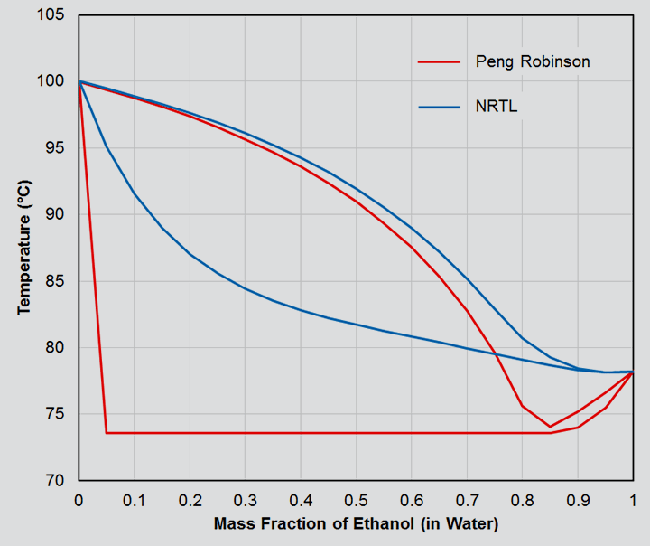
The NRTL results match experimental data very closely, and show smooth changes over the composition range, whilst also predicting the azeotrope at just over 95% ethanol by mass.  It follows that the compositions of the different phases will also transition smoothly and correctly across the range.

By contrast, the results from Peng Robinson predict the same bubble point temperature across the majority of possible compositions, and as a result, the vapour/liquid compositions within the two phase region will be heavily skewed.  In addition, two liquid phases are predicted despite ethanol and water being highly miscible under these conditions.

Whilst these differences may stand out when viewed holistically, the danger creeps in during day to day use when you are more likely to be looking at a single composition in isolation.  As such, the errors which are clearly seen in Figure 1 are far less obvious.  For a 30 wt% ethanol system, would you really pick up that the bubble point was being simulated as 73.5°C rather than 84.5°C?

A second example of the effect of fluid package choice can be seen when considering a sulfuric acid and water mixture.  Liquid acid systems can behave very differently to a thermodynamically ideal liquid due to the disassociation of ions, which results in local concentrations of each component on a molecular level.  Specialist fluids packages such as Electrolyte NRTL are designed to capture this non-ideality: an AspenPlus simulation using this package predicts the boiling point of 75 wt% sulfuric acid to be 184.4°C, comparing favourably with the experimental boiling point of 185°C.  In this case, Peng Robinson misses the mark, and would predict a boiling point of 108.7°C.

Once again, would you intuitively question the Peng Robinson boiling point as suspect if it was considered in isolation with no comparison against more suitable methods or experimental data?

Moving away from fluid packages, another example of a ‘less than obvious’ error arising from the use of simulation software is modelling pipe segments in Aspen HYSYS.  Unfortunately, the option to check for choked flow is not enabled by default.  As a result, there is no realistic upper limit on the velocity and no pressure discontinuities will be predicted.  The author has seen significant errors incorporated into a calculation as a result of not checking this option; the absence of pressure discontinuities meant that the pressure seen by a vessel in the middle of a modelled system was predicted much lower than it should have been.

Another slightly ‘hidden’ option is associated with RadFrac columns in Aspen Plus.  The user can select to solve the block in either “equilibrium” or “rate-based” mode; the difference being whether the time for mass and heat transfer to occur is considered.  Keeping the default setting of “equilibrium” (which assumes full thermodynamic equilibrium is reached at each stage) generally solves much faster, but can miss the mark significantly when compared to how the actual system responds.  For a system where the column sump temperature is controlled by recycling some of the bottom liquid product to the top of the column via a cooler, the two solver methods differ significantly.  In equilibrium mode, 224 m³/h of recycle is required compared to just 147 m³/h needed in rate-based mode.  Comparison against actual plant data shows the rate-based mode answer to be much closer to how the real system runs.

The examples considered above highlight the fact that simulation software heavily relies on the user asking the right questions to begin with – the software can only carry out heat and mass balances based on this input.  It should therefore be a prerequisite for engineers to fully understand what they have input to the model, and to critically challenge the output.

Where did the pressure come from?

Another way in which simulation software can be misused is by ‘accidentally’ creating mass and energy.  Being able to simply type a set of conditions into a box makes it very easy to do this despite good intentions.  It is this error which underpins the main problems that the author has seen when using software as part of pressure relief calculations.  Manipulation of simulations should reflect as accurately as possible how a real system would act, which for pressure relief can be generally encompassed and tested for by asking the question “where did the pressure come from?”, as a simple but powerful test as to the validity of the method.

Generally speaking, the only ways for a real system to increase in pressure is for there to be more mass entering than is leaving, more energy being added or created than is being lost or removed, or perhaps some combination of the two.   It goes without saying that the extra mass or energy flowing into a vessel must come from somewhere else in the system since it cannot be spontaneously created.  However, this is what the author has seen happen in simulation software, where thermodynamics can be played with fast and loose resulting in perhaps sensible or plausible looking results, that are physically impossible to reach or create in real life.

To illustrate these errors, let us consider a simple pressure relief example.

A simple example – Vapour relief from a separator vessel

Let us consider a pressure relief scenario for a two-phase separator.  As is common with pressure relief scenarios, we will consider the outlet to the system in question to be closed.  The source of mass flow into the separator is from a higher pressure system upstream of the separator via a control valve that has failed or become stuck in an open position.

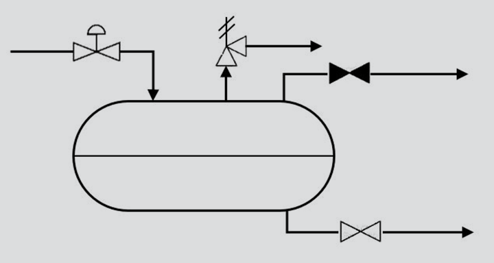
Under normal operation, the separator will disengage the liquid and gas into two streams with compositions determined by the thermodynamic equilibrium of the mixture, which is dependent on the temperature and pressure of the separator.  During the relief scenario, the pressure in the vessel will rise until it is limited by the relief valve (assuming it is correctly sized and works as expected).  The key point in this set up is that the increased pressure in the vessel will result in a new chemical equilibrium being established, thus the gas and liquid will have different compositions and therefore different physical properties compared to steady state conditions.

Dependent on the system under study, the difference in pressure between normal operation and a relief valve lifting varies significantly.  The author has seen cases where the gap is significant: normal flowing pressure at 15-20 barg, and relief pressure at over 90 barg.

It is also worth paying attention to how the temperature of the system could change as the pressure increases.  In our example, as pressure drops over the control valve, there will be a cooling effect (disregarding examples such as hydrogen where Joule-Thompson coefficients are negative resulting in temperature increases).  For this scenario, the upstream pressure remains constant, and so the pressure drop across the failed control valve will decrease as the pressure rises in the two-phase separator.

Looking at the effect of pressure and temperature qualitatively, the increasing pressure will cause heavier components in the vapour to condense, resulting in a lighter molecular weight vapour.  The concurrent increase in temperature caused by the reduced pressure drop across the control valve will act to promote lighter components in the liquid phase into the vapour phase, resulting in a heavier overall vapour.  Since these effects are simultaneous and compete in terms of their effect on the system, it quickly becomes non-intuitive to predict how the system will respond.

Therefore, it is important to correctly model the effects of temperature and pressure in a simulation to capture the, perhaps, unexpected behaviour.

Incorrect modelling practice

Relating to the simple example above, the most common way that the author has seen simulations being incorrectly manipulated, it to give no consideration to the effect of the equilibrium in the separator at the relief conditions.  Generally, a copy of the vapour outlet stream is made at its normal conditions.  The user then carries out what can only be termed as a “magic pressure rise”, by either typing in a new pressure directly into the new stream, or by passing the stream through a valve or other pressure changer resulting in a second new stream at the relief pressure.

Simply typing over a value should never be a method to simulate a real system, as this will change the overall enthalpy of the stream and as a result, energy has been created or destroyed.  Passing the stream through a valve or similar block is marginally more realistic, as the software will carry out an adiabatic flash and adjust the temperature of the stream accordingly such that the change in energy resulting from the pressure change is cancelled out.

However, neither of these methods represent the actual system due to the lack of inclusion of the separator.  As a result the overall composition remains unchanged before and after implementing the pressure rise.  The correct way of modelling this scenario starts with asking the question posed earlier in this article – where has the pressure come from?

How should this example be modelled?

In this example, the pressure is coming from the higher pressure in the upstream vessel.  Therefore, this should be the starting point for manipulating the simulation, not the vapour outlet from our two-phase separator which might seem like the more intuitive beginning.  A copy of this upstream higher pressure stream should be taken, and then the rest of the system modelled as it happens in the real system.

First the copy of the higher pressure stream should have its pressure dropped adiabatically to the relief pressure of the two phase separator; this represents the change over the failed control valve.  By virtue of being adiabatic, no energy will be created or destroyed, and any Joule-Thompson effect cooling will be properly captured.  Next, a separator block should be used to split the vapour and liquid components that will have resulted.  Since the two phases are being split from a stream which is at the correct conditions for the relief scenario, the equilibrium will have been correctly established, and so changes in composition resulting from the abnormal temperature and pressure are captured.  The resulting vapour stream can now be used to represent the properties of the fluid that will be relieved by the relief valve.

This method only involves a couple of extra steps over the marginally quicker, but incorrect methods discussed.  However, the result is a model which represents a thermodynamically possible change.

Impact of modelling methods

An example which demonstrates the effects of modelling “magic pressure rises” comes from a pressure relief validation project for an offshore oil and gas platform.  The setup matches the example already discussed with a high pressure separator feeding a lower pressure separator via a control valve.

Carrying out the manipulation the incorrect way by simply raising the pressure of the normal operating condition vapour stream via an adiabatic flash results in a vapour molecular weight of 21.5 kg/kmol and a relief temperature of 50°C.  In addition, a small amount of liquid phase is predicted as the pressure of an already saturated stream has been increased; this liquid phase is generally ignored by the user to obtain just the vapour properties.  Despite this example being a vapour relief case from a separator, the author has seen all too often this liquid phase being disregarded; a red flag that the user is not asking the right questions of the simulation.

Correctly manipulated, starting from the high pressure upstream vessel, and flashing the stream at the relief conditions, the molecular weight of the relief vapour is 19.9 kg/kmol and the temperature is 43°C.  Delving into more details, the lower molecular weight is predominantly down to the reduction in the mass fractions of C2-C5 gases, whose mass fractions are reduced by approximately 40% relatively.  There is a corresponding relative 8% increase in the methane mass fraction.  These composition shifts fit with a qualitative analysis of the scenario, with heavier hydrocarbon gases condensing resulting in a lighter more methane rich vapour.

What isn’t intuitive is the effect on non-hydrocarbon gases within the stream, with carbon dioxide and hydrogen sulphide fractions decreasing whilst the nitrogen fraction increases.  The water fraction is also significantly affected, with the correctly manipulated stream containing half as much water.

So what is the impact of these differences on engineering calculations?  For this example, the difference in temperature and molecular weight would result in a required relief valve orifice area approximately 3% different for a vapour relief sizing.  However, the most significant impacts are more wide spread.  Since the incorrect stream is not a saturated vapour composition, any further modelling that uses that composition e.g. inlet and outlet piping pressure drops, flare/vent system, could be more significantly affected as flow will likely become two-phase and increase pressure drops.

The author has seen errors in the water composition as a result of magic pressure rises have significant effect on studies regarding ice and hydrate formation within flare header pipework.  These studies used the total flowrate along with the water composition of a relief stream to work out how long it would take to block a section of pipework if it is sufficiently cold for solids to form.  The time to block is calculated and is directly proportional to water composition so whilst a 1% to 0.5% mass fraction change seems insignificant, it could halve the time required for a blockage to form.  This is often the difference between an urgent high priority finding requiring quick action, and a lower priority finding that may result in no further actions.

More complex pressure relief scenarios

The above example is a simple, albeit common setup for a pressure relief calculation.  However, the general principle of following where the pressure is coming from applies to more complex systems as well.  For example, a gas compressor system where the pressure relief event is a blocked discharge.  Clearly the compressor is a source of pressure, but the source of suction pressure also needs to be considered.

The author has seen cases where a suction pressure higher than normal operating is necessary such that the compressor discharge is able to reach the relief point.  As a result, the upstream separator would need to be at higher than normal pressure conditions, and so the model should be built to incorporate this.  The difference in molecular weight and temperature caused by this upstream change will need to be considered by the model to alter the compressor curves accordingly.

In other cases, minimum flow recycle lines around the compressor come into play.  The increased outlet pressure during the relief event results in a larger cooling effect as this pressure is dropped through the minimum flow recycle line compared to normal operation.  This can be enough to significantly reduce the compressor inlet temperature as the recycle mixes back in with the normal supply gas.  As a result, the equilibrium compositions will be altered in any suction knock out vessels.  This combined with the cooler temperature will affect the volumetric flow of the compressor suction, and therefore alter the operating point on the flow curve.  Simulations of compressors are often used to determine the required relief rate for a relief valve and the cumulative effect of the discussed events should be included in a model as they could have a large impact on any sizing calculations.

Further, models of compressor systems are likely to be built such that the simulation follows the characteristic flow curve (and sometimes the efficiency curve) of the equipment, and are unlikely to include any other information such as supplied motor power.  As such, it is good practice to question the power supply predicted by the model.  Remember that the simulation will simply supply as much power as is needed to match the inlet and outlet conditions requested.  The author has seen pressure relief cases that have not performed this check, and as such carried out calculations for impossible cases.  If the simulation power required does exceed the possible supply on the equipment, then the model should be manipulated so that the power requirement is limited; this may also have the effect of removing a scenario as a credible relief case.

Conclusions

Process simulators are powerful tools which enable engineers to model a wide variety of systems, and obtain useful data at conditions which would be too hazardous to test on a real system.  However, behind the scenes, the main ‘intelligence’ of the software is to carry out mass and energy balances purely based on the inputs which it has been given.  It follows, that providing the wrong inputs, is likely to result in a flawed output.

Users should always keep in mind that they are producing a model of a real system, and must therefore ask questions of the simulator that represent that system.  Part of this relates to understanding the effect of the numerous options that are presented to the user at all stages of modelling, whether it be choice of fluid package or asking the software to predict real world effects such as chokes in gas systems, or mass transfer limitations.

It is equally important to manipulate the inputs and streams of the model correctly, as to steer the mass and energy balances towards how a real system would respond.  Much of the battle to achieve this is conquered by keeping a mindset to always capture the physical effects that would occur on a real plant, and not to shortcut them.  For pressure relief purposes, simple checks such as asking oneself “where is the pressure coming from?” can be all that is needed to prompt correct use of the software and avoid creating unrealistic ‘magic pressure rises’.

By keeping the correct mindset when using modelling software, the quality of the output will significantly increase, with very little extra effort and time.