Practical Process Control Part 8: Determining Tuning Constants for Tight and Averaging Level Control

Myke King continues his detailed series on process control, seeking to inspire chemical engineers to exploit untapped opportunities for improvement

In the previous article we showed how to determine the parameters necessary to calculate level controller tuning. These are: 

V= working volume of the vessel

d = maximum acceptable deviation from setpoint (40% in our example)

f = normally expected flow disturbance

F = flow when the level controller output is 100%

ts = level controller scan interval

We now need to determine the values for controller gain (K_c), integral time (T_i) and derivative time (T_d).

Tight control

To design the controller to deliver tight control, we start with a proportional-only controller – where E is the deviation from setpoint (the error) and M the controller output.

Assuming that the process before the flow disturbance is at steady state, then E_n-1 will be zero. After the disturbance, the error (in dimensionless form) is given by the change in liquid volume as a fraction of the working volume.

For the level to stop moving, the controller must adjust the outlet flow by the same amount as the inlet flow. Again, in dimensionless form

For tight control, we design the level controller to correct the imbalance in the shortest possible time. This is at the end of the first scan interval, so the maximum controller gain is given by

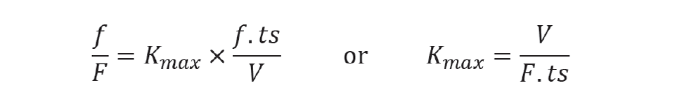
Care should be taken in consistency of engineering units. For example, if F is in m³/h, then V must be in m³ and ts in hours. Note that the result excludes f. Whatever disturbance is made to the inlet flow, one scan interval later, the controller will do the same to the outlet flow. With a proportional-only controller there will be an offset from the level setpoint. It will be negligibly small but, if required, integral action can be included. To determine this, we first calculate the vessel time constant (T). This is defined as the time taken, with no controller in place, for the level to reach the maximum deviation (d) when the inlet flow is changed by f. This is given by

For tight level control, we choose a small value for d, say 1%. Empirically, setting the integral time (T_i) to 8T gives good control. We must again be careful with units. Depending on the control system, T (and hence T_i) should be in minutes or seconds. Because we have included integral action, we must slightly reduce the proportional action. Again, empirically, setting K_c to 0.8K_max works well. Only in unusual circumstances (that we’ll cover in the next issue) does level control benefit from derivative action. Full controller tuning is therefore

Unlike most controllers, the tuning of tight level control is particularly sensitive to the scan interval. For example, if the current system scan interval is one second and is increased to two seconds, the gain of all tight level controllers should be halved.

There are other factors that might limit the maximum gain the controller will support – most notably noise. It may be necessary to reduce K_c to avoid excessive control valve movement.

Averaging control

We take much the same approach to designing an averaging level controller, starting with a proportional-only controller.

But this time we design the controller to operate as slowly as possible. We define the minimum controller gain (K_min) as that which will leave an offset of d. In other words, the level will move to the nearest alarm limit and stay there. By doing so, we use all the available surge capacity. Clearly not a practical controller, we will later add integral action to bring the level slowly back to setpoint.

As in the tight control case, the averaging controller must match the outlet flow to any change in inlet flow. But, unlike the tight controller, this takes place slowly – involving a large number of controller scans.

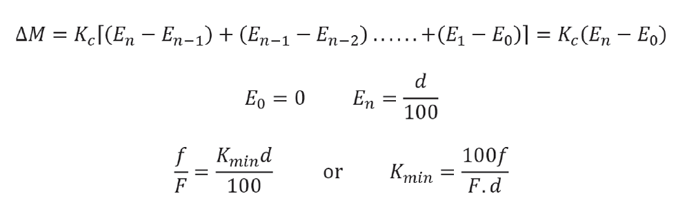
We apply the same empirical method, as we did for tight control, to give full controller tuning as

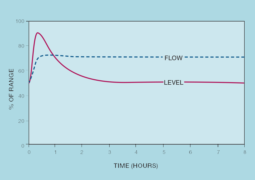
Figure 1 shows how this controller responds. In this example, avoiding the alarm at 90%, it takes around 30 minutes for the downstream flow to reach its new value, as opposed to the few seconds taken with tight control. This will substantially improve the stability of any downstream unit. It does, however, require that the level be away from its setpoint for over an hour; it is this that the process operator might find difficult to accept.